Risk-Neutral Pricing & No-Arbitrage
Objectives
- State the no-arbitrage principle, the law of one price, and replication as the engine of derivative pricing.
- Define an equivalent martingale measure Q and write risk-neutral pricing as a discounted expectation.
- Write the risk-neutral SDE (drift μ → r) and the market price of risk that Girsanov's change of measure absorbs.
- Explain the two equivalent routes to a price — the delta-hedge PDE and the discounted expectation — and connect them to the SVQ fair-value service.
You know how to model a price as it wanders. What you cannot yet do is attach a fair number to a claim written on it — an option, a forward, anything whose payoff depends on where the price ends up. The surprising fact, and the heart of this chapter, is that you can do it without ever predicting where the price will actually go. That sounds impossible. It is the deepest idea in derivatives pricing, and once you see it you will never read a fair value the same way.
No-arbitrage and the law of one price
Start with a principle so simple it feels trivial: no arbitrage. An arbitrage is a free lunch — a trade that costs nothing today, can never lose, and sometimes wins. In a functioning market such trades do not persist: the moment one appears, someone exploits it, and the exploiting moves prices until the free lunch closes. So we assume, as a modeling axiom, that no free lunch exists. This is not a claim about psychology or efficiency — it is a much weaker, much more reliable thing: a constraint on which prices are mutually consistent.
Watch what that single constraint forces. Suppose you can build two portfolios that pay out exactly the same amount in every future state of the world — one an option, the other a recipe of stock and cash that mimics the option's payoff. Then they must cost the same today. Because if one were even a penny cheaper, you'd buy the cheap one, sell the dear one, pocket the difference, and hold a position that nets to zero forever — an arbitrage, which we forbade. This is the law of one price, and it is the engine under every fair value the platform shows.
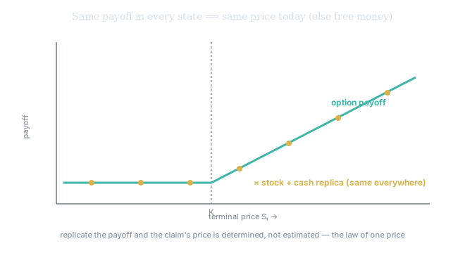
Figure 1. A call's payoff and a stock-plus-cash replica that matches it in every terminal state. Because they pay identically everywhere, no-arbitrage nails their prices together today. The claim's price is therefore determined — not estimated — by the cost of the replicating recipe.
Replication
The trick of pricing, then, is replication: if you can copy a claim's payoff with simpler instruments whose prices you know, the claim's price is fixed by the cost of the recipe. You never forecast the asset — you only copy the payoff. Doing this by hand for every claim would be brutal, so there is a far more powerful way to say the same thing, through a change of probability.
The martingale, and the measure Q
Consider the discounted price of a tradable — its price divided by the growth of a risk-free bank account, . Under the real-world probabilities , this tends to drift, because risky assets earn more than cash to compensate for risk (that excess is the risk premium — the VRP you met in 201). Now ask a strange question: is there some other set of probabilities — a re-weighting of the same future states — under which the discounted price has no drift, i.e. is a martingale, its expected future value equal to today's?
The fundamental theorem of asset pricing says yes, and sharply: a market is free of arbitrage if and only if there exists at least one such measure. We call it an equivalent martingale measure — the risk-neutral measure. Two words carry the weight. Martingale: under the discounted tradables have zero drift — the risk premium is engineered away. Equivalent: agrees with the real world about which events are possible (any state gives positive probability, does too, and vice versa) — it may disagree wildly about likelihood but never about possibility, which is exactly what blocks conjuring an arbitrage through an impossible-event loophole.
Risk-neutral pricing: one line
With in hand, pricing collapses to a single line. The fair value today is the discounted expected payoff under :
Compute the average payoff using the risk-neutral probabilities, discount at the risk-free rate, done. No risk premium appears anywhere. The asset's true expected return — the thing you spent a career trying to forecast — has vanished from the pricing formula. It got absorbed into the moment the drift was removed.
The risk-neutral SDE and the market price of risk
Here is the operational content of "the drift vanished." Under the real world the stock follows . Switching to changes the drift — and only the drift — from to the risk-free rate :
The volatility is untouched (it is a real, observable property of the paths); the drift is rewritten. The bookkeeping that does this is Girsanov's theorem: define the market price of risk
and is a Brownian motion under under which the drift becomes . That — excess return per unit of volatility, a Sharpe-ratio-like quantity — is precisely the risk premium, and re-weighting the probabilities zeroes it out.
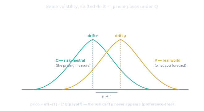
Figure 2. The two worlds. Under P the terminal price is centered at the real drift (your forecast); under Q it is shifted to drift (the pricing measure) — same volatility, different center. Pricing takes the expectation under the teal Q-distribution and discounts. Forecasting lives under P; pricing lives under Q, and they are not the same act.
Two routes to the same price
You have now seen pricing from two directions, and they are the same mountain. Route 1 (last chapter): apply Itô to the option, delta-hedge away the , and the risk-free portfolio must earn — giving the deterministic Black-Scholes PDE for . Route 2 (this chapter): change to and write the discounted expectation . The Feynman-Kac theorem proves these give the identical number: the solution of the PDE is that expectation. And when the expectation has no closed form (path-dependent, exotic), you compute it by simulation — the Monte Carlo of Module 202-6, run under .
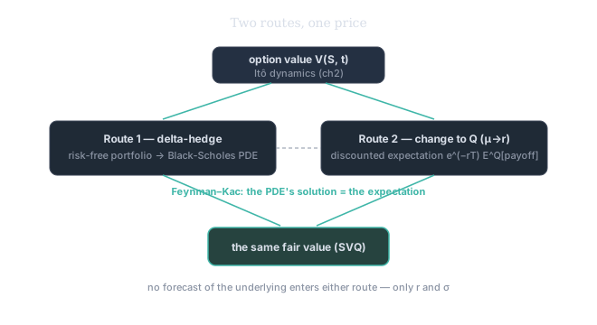
Figure 3. One price, two derivations. Delta-hedge to the PDE, or change measure to the discounted expectation — Feynman-Kac links them. Notice what enters neither route: any forecast of the underlying. Only and .
This is why risk-neutral pricing is preference-free: two investors who violently disagree about how much the asset will rise, and how much risk they can stomach, must still agree on the option's price — provided both refuse a free lunch. The disagreement lives in the real measure; the price lives in . And a warning that matters for the rest of the institute: the risk-neutral probabilities are a pricing device, not a forecast. The -probability of an up-move is not your honest belief the asset will rise. Pricing a thing and having an edge on it are different questions — keep them apart.
The SVQ fair-value service, run on a liquid option, returns a discounted risk-neutral expectation: SVQ takes the spot, the risk-free rate, the time to expiry, and an implied-volatility surface, then prices the claim as . Just as telling is what is absent from the inputs — no field for the asset's expected return, no drift, no view. That is not an oversight; it is the theorem at work: the fair value is the cost of replication, and replication never needed a forecast. When SVQ's fair value diverges from the screen price, the gap is not a prediction the asset will move — it is a no-arbitrage statement that something in the inputs disagrees with the market, and (since and are known) that something is almost always : the market's implied volatility. That gap is a candidate for evidence; which way the asset actually goes is a separate question.