Black–Scholes–Merton & d1/d2
Objectives
- State the Black–Scholes–Merton formula for a European call and put and identify what each input controls.
- Define d1 and d2, explain why they differ by exactly σ√T, and read each as a probability-flavored quantity.
- State put-call parity, and explain implied volatility as inverting the formula for σ.
- Trace how SVQ turns spot, strike, rate, time, and volatility into one fair value, and where a disagreement really lives.
By the end of the last chapter you had geometric Brownian motion, Itô's lemma, and the risk-neutral argument that lets you price by replication — the fair value is . Now we cash all of it in. We are going to evaluate that expectation for a European call and out will fall the single most famous formula in finance — the one SVQ computes every time it prints a fair value — and take it apart until the two mysterious symbols inside it, and , stop being letters and start being meanings.
The intuition: two competing pieces
What is a European call worth? At expiry it pays the amount by which the stock finishes above the strike, and nothing if it finishes below. So its value today is two competing pieces: on the upside you receive the stock — but only in the worlds where you exercise; on the downside you pay the strike — again only where you exercise. A fair price is the present value of the first minus the present value of the second. Black–Scholes is that sentence made precise under the risk-neutral measure.
The call formula
Evaluate the risk-neutral expectation over the lognormal terminal price (Modules 102-2, 301-3) and you get
where is the standard-normal CDF (Module 102-1) — for any number it returns the probability a standard normal lands below it, always between 0 and 1. Those two terms are the weights on the two pieces. is, under the risk-neutral measure, the probability the call finishes in the money and you actually pay the strike. is subtler — the probability of exercise re-weighted by how much stock you receive, which turns out to be the option's delta. So the structure is exactly the sentence above: expected stock received, minus expected strike paid, each discounted.
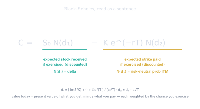
Figure 1. Black–Scholes as a sentence: is the discounted expected stock you receive if you exercise; is the discounted expected strike you pay. is the risk-neutral chance of exercise; is the delta.
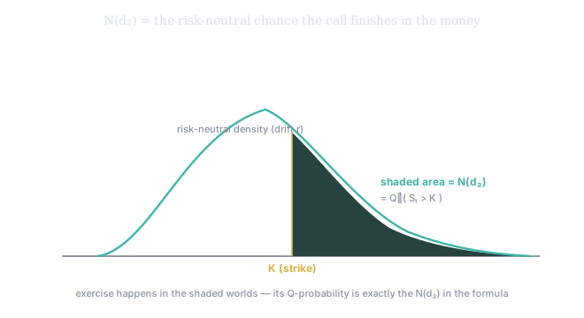
Figure 2. is an area: take the risk-neutral terminal-price distribution (drift , from ch3) and shade the region above the strike. That shaded probability — — is exactly the sitting in the formula.
d₁ and d₂
Here is the anchor of the chapter, the exact expressions SVQ uses:
Read the numerator of left to right and it tells a story. is your moneyness — how far in or out of the money, in the log space you learned to trust (zero if spot equals strike, positive in-the-money). To it we add : the is the risk-neutral drift (the stock grows at the risk-free rate, pushing a call toward exercise), and the is the Itô correction you derived in ch2 — the signature of moving a convex function through GBM, not optional and not a fudge. Divide the whole thing by , the standard deviation of the log-return over the option's life, and becomes a distance in standard deviations: how many sigmas of cushion stand between you and the strike, with the drift leaning in.
That makes almost obvious — exactly one standard deviation of terminal uncertainty. Hold it this way: governs whether you exercise; governs how much stock you walk away with when you do; volatility is the wedge between them. When is tiny they nearly coincide and the option behaves like a forward; when is large the wedge opens and the value comes increasingly from the payoff's asymmetry.
The put, and put-call parity
The put follows from the same machinery — or, for free, from put-call parity, a model-independent no-arbitrage identity: a call minus a put (same strike and expiry) replicates a forward, so
Same two characters, mirrored. Parity is worth memorizing because it holds whatever model is right — it is pure no-arbitrage, so any pricer that violates it (SVQ's included) has a bug.
Five inputs, one unknown: implied volatility
Notice what the formula needs: spot, strike, rate, time, and volatility. Four you read straight off a screen. The fifth, , is the only genuine unknown — which is why every interesting question in the rest of this tier is a question about . And because the call price is strictly increasing in (more volatility can only help an option), the map is invertible: given a market price , you can solve
and the unique answer is the implied volatility — the market's own estimate of future volatility, read backwards out of the price. This inversion is the single most-used operation in options, and when you do it strike-by-strike and find the answer is not one constant number, you have discovered the volatility surface — exactly where the next chapter begins.
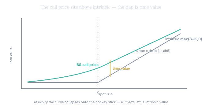
Figure 3. The call price as a function of spot sits above the intrinsic hockey-stick ; the vertical gap is time value, and the curve's slope is delta (the first Greek, ch5). As expiry approaches, the curve collapses onto the hockey-stick — time value decays to zero.
A worked value
SVQ prices a near-the-money call like this one: spot , strike , rate , expiry years, implied volatility . Then . The numerator of is , so and . Reading the normal CDF, and , so That single number on the SVQ panel is this arithmetic. When SVQ flags an option as cheap or rich, it is comparing the market price to this fair value — and the entire disagreement lives in the it was fed (equivalently, in the implied vol the market is quoting back).