Itô's Lemma & Stochastic Differential Equations

In the last chapter you met Brownian motion — the idealized walk whose increments are independent, Gaussian, and whose roughness never smooths out no matter how closely you zoom. Now you must do calculus on it. And the first thing to accept is that ordinary calculus, the calculus of smooth curves you learned years ago, does not bend here. It breaks.

Here is the intuition before any formula. Ordinary calculus rests on a quiet assumption: over a tiny step $dt$ , the change in a smooth function is proportional to $dt$ , and its square is proportional to $dt^2$ — so much smaller that we throw it away. That throwing-away is the whole game of classical calculus. But a Brownian path does not move proportionally to $dt$ . Over a tiny step it moves like $\sqrt{dt}$ , because its variance grows linearly with time (ch1). So when you square a Brownian increment you do not get something negligible — you get something of order $dt$ , exactly the order you were keeping. The second-order term refuses to vanish.

The multiplication table

We captured this in ch1 as the quadratic variation, $(dW)^2 = dt$ . It comes with two companions — since $dt$ is already tiny, anything of higher order dies:

$(dW)^2 = dt, \qquad dt\,dW = 0, \qquad (dt)^2 = 0.$

Read it slowly: the square of the random part survives, and survives as an ordinary, deterministic $dt$ . This is the multiplication table of stochastic calculus, and everything follows from it.

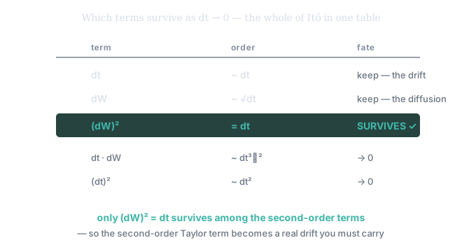
*Figure 1.* Of all the terms in a Taylor expansion, only three matter as $dt \to 0$: the drift ($dt$), the diffusion ($dW \sim \sqrt{dt}$), and — the whole novelty — the squared Brownian increment, which does *not* vanish but equals $dt$. That single survivor is the entire content of Itô calculus. — *Figure 1.* Of all the terms in a Taylor expansion, only three matter as $dt \to 0$ : the drift ( $dt$ ), the diffusion ( $dW \sim \sqrt{dt}$ ), and — the whole novelty — the squared Brownian increment, which does *not* vanish but equals $dt$ . That single survivor is the entire content of Itô calculus.

The stochastic differential equation

Now describe how an asset moves. A stochastic differential equation (SDE) says the change over the next instant is a predictable part plus a random part:

$dX = a\,dt + b\,dW.$

The $a\,dt$ is the drift — the steady pull, where the process tends to go on average. The $b\,dW$ is the diffusion — the shock delivered by Brownian motion, and the only term carrying randomness. Every pricing model is, at bottom, a choice of those two functions. The most important choice in finance is geometric Brownian motion, where drift and diffusion are both proportional to the asset's own level:

$dS = \mu S\,dt + \sigma S\,dW.$

The asset drifts upward at a constant percentage rate $\mu$ and is shocked by a percentage volatility $\sigma$ , both scaled by the current price. This is the assumption under Black–Scholes and inside every SVQ pricing model, and it encodes one belief: that returns, not prices, behave randomly and stationarily — the log-return world of the foundations course.

Itô's lemma: the corrected chain rule

Now the centerpiece. Take a function of your process — the log of the price, or the value of an option that depends on it — and ask how it changes. In ordinary calculus you'd use the chain rule and stop at the first derivative. Here you cannot, because the second-order term does not vanish. Itô's lemma is the corrected chain rule: for $G = f(X,t)$ with $dX = a\,dt + b\,dW$ ,

$dG = \left(\frac{\partial f}{\partial t} + a\,\frac{\partial f}{\partial X} + \frac{1}{2}\,b^2\,\frac{\partial^2 f}{\partial X^2}\right)dt \;+\; b\,\frac{\partial f}{\partial X}\,dW.$

Everything except one term is the ordinary chain rule. The extra piece, $\tfrac12 b^2 f_{XX}\,dt$ , is born entirely from $(dX)^2 = b^2(dW)^2 = b^2\,dt$ — a genuine, non-negligible drift you must carry, conjured out of pure randomness.

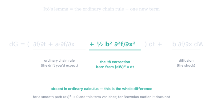
*Figure 2.* Itô's lemma, decomposed. The drift and diffusion are what ordinary calculus would give — but the highlighted $\tfrac12 b^2 f_{XX}\,dt$ term has no classical counterpart. It exists only because $(dW)^2 = dt$. Strip it out and you have the chain rule from school; keep it and you have finance. — *Figure 2.* Itô's lemma, decomposed. The drift and diffusion are what ordinary calculus would give — but the highlighted $\tfrac12 b^2 f_{XX}\,dt$ term has no classical counterpart. It exists only because $(dW)^2 = dt$ . Strip it out and you have the chain rule from school; keep it and you have finance.

The volatility drag, derived

Let it bite. Take geometric Brownian motion and ask what the log of the price does — the transformation you care about, since you live in log-returns. With $f = \ln S$ : $f_S = 1/S$ and $f_{SS} = -1/S^2$ . Feed these in with $a = \mu S$ , $b = \sigma S$ . The first-order part gives $\mu\,dt + \sigma\,dW$ ; the Itô term gives $\tfrac12(-1/S^2)(\sigma^2 S^2)\,dt$ — the $S^2$ cancels — leaving $-\tfrac12\sigma^2\,dt$ . So

$d\ln S = \left(\mu - \tfrac{1}{2}\sigma^2\right)dt + \sigma\,dW.$

That $-\tfrac12\sigma^2$ is the celebrated variance drag (or Itô correction). It is not a fudge factor — it is the analytic reason a volatile asset with positive expected return can see its typical path drift lower than its average suggests: volatility itself eats into compounded growth. You met this in the foundations course intuitively (a 50% loss needs a 100% gain back) and stated it as a fact in 102; here is its exact source. And because $\ln S$ has constant drift and diffusion, you can integrate it directly to the closed-form solution of the GBM SDE:

$S_t = S_0\,\exp\!\left(\left(\mu - \tfrac{1}{2}\sigma^2\right)t + \sigma W_t\right),$

which is lognormal — closing the loop back to Module 102-2, where you took this shape on faith. Now you have derived it.

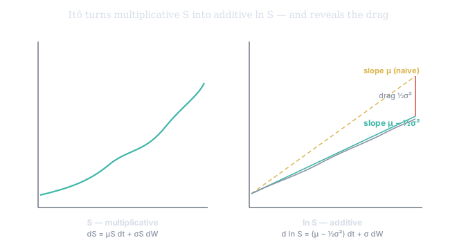
*Figure 3.* Itô turns the multiplicative price $S$ (left) into the additive log-price $\ln S$ (right), whose drift is $\mu - \tfrac12\sigma^2$ — visibly *below* the naive $\mu$ line. The gap between them, $\tfrac12\sigma^2$, is the drag, and it is exactly the $-\tfrac12\sigma^2$ the Itô term produced. — *Figure 3.* Itô turns the multiplicative price $S$ (left) into the additive log-price $\ln S$ (right), whose drift is $\mu - \tfrac12\sigma^2$ — visibly *below* the naive $\mu$ line. The gap between them, $\tfrac12\sigma^2$ , is the drag, and it is exactly the $-\tfrac12\sigma^2$ the Itô term produced.

This is the institute's throughline made rigorous: separating the drift you can lean on from the diffusion that is just noise, and knowing precisely how much of an observed move was signal versus the unavoidable, self-generated drag of randomness.

In Saqrid

Every option price SVQ shows you is the solution to a partial differential equation that Itô's lemma produces. Applied to an option value $V(S,t)$ , the lemma exposes a $dW$ shock that the right holding of the underlying hedges away — the random term cancels exactly because $V$ and $S$ are driven by the same Brownian motion. What remains, with no randomness left, is the Black–Scholes PDE, and its solution is the number on the SVQ pricing panel. So the $-\tfrac12\sigma^2$ you just derived is not academic trivia — it is literally the term that makes the model's theta and implied-vol surface come out right. When a SVQ price disagrees with the market, the disagreement is about $\sigma$ , the diffusion coefficient in this very SDE. (The full derivation is next chapter.)