From Random Walks to Brownian Motion
Objectives
- Construct a scaled random walk and take its continuous-time limit to recover standard Brownian motion.
- State the three defining properties of Brownian motion and explain why the increment's standard deviation scales as √t.
- State the quadratic variation (dW)² = dt and explain why it breaks ordinary calculus and forces Itô calculus.
- Write the generalized Wiener process dX = a·dt + b·dW as the drift-plus-diffusion skeleton of every price model.
You already know how to think about a single return. Now you need to think about a whole path. A price does not move once and stop — it moves, and moves again, and the moves pile into a trajectory through time. To put a probability on where an asset might be tomorrow, or at expiry, you need a mathematical object that produces random paths. The object nearly every option-pricing model is built on — the one under the diffusion SVQ assumes — is Brownian motion. And the cleanest way to understand it is to build it yourself, from something almost insultingly simple: a coin flip.
The random walk
Picture a particle at zero. Each step, flip a fair coin: heads it moves up one, tails down one. The position after flips is the running total,
This is the simple random walk, the ancestor of everything here. Where do you expect the particle to be after many flips? On average, back at zero — the ups and downs cancel in expectation, . But you would be a fool to bet it is at zero. The interesting quantity is not where it tends to be but how far it tends to wander, and that has a precise signature: since the flips are independent and variance adds for independent things,
Variance grows linearly with steps, so the typical distance grows like the square root of the number of steps. Four times as many flips, only twice as far from home. Hold onto that square root — it is the single most important fact in this chapter, and the reason a quiet market and a violent one are not as different as they look.
The scaling limit → Brownian motion
Now turn the coin-flip toy into a continuous process. Squeeze time and shrink the steps: take many flips per second, and — to stop the particle flying off to infinity — make each step smaller. The recipe the square-root law demands is exact: if the time between flips is , make each step's size equal to . Take more and smaller, and pass to the limit. What survives is a continuous random path — standard Brownian motion, the Wiener process — whose increment over a small step is
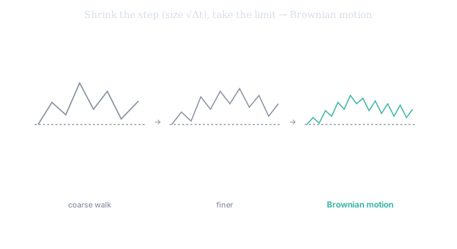
Figure 1. The limit in three frames: a coarse few-step walk, a finer one, and — as the step shrinks with size — the continuous, infinitely-jagged Brownian path. Every price model in this course is dressed-up version of that right-hand object.
The three defining properties
Strip away the construction and Brownian motion is pinned down by three properties.
One — it starts at zero: (a convention, but a useful one).
Two — its increments are independent and Gaussian. Over any stretch from to ,
so the change over an interval of length has variance and standard deviation — the square-root law, now exact. And non-overlapping increments are independent: the future change knows nothing about the past. The process has no memory.
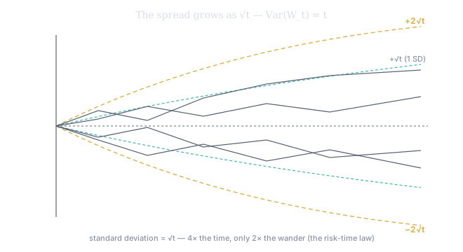
Figure 2. Because , a bundle of paths spreads from the origin inside a envelope — the standard deviation growing as the square root of elapsed time. This parabola-shaped cone is the risk-time law you met as √252 annualization, drawn in continuous time.
Three — its paths are continuous but nowhere differentiable. The particle never teleports — you can draw the trajectory without lifting your pen — yet that trajectory is so jagged it has no well-defined slope anywhere. It wiggles at every scale you zoom into, infinitely. That roughness is not a defect; it is precisely what makes ordinary calculus fail on these paths — which is the whole reason this course exists, and which we can now make exact.
The strange arithmetic: quadratic variation
Here is the fact that separates stochastic calculus from the ordinary kind. Chop into tiny steps and add up the squared increments. For a smooth function , each increment is , so , and summing of those vanishes as you refine — the squared wiggles of a smooth curve go to zero. But for Brownian motion, with , so each squared increment is about , and summing of them gives
This is the quadratic variation, and it is astonishing: the squared wiggles do not vanish — they accumulate to a deterministic .
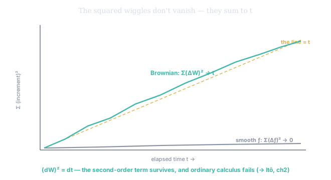
Figure 3. Accumulate the squared increments. A smooth function's sum collapses to zero; Brownian motion's climbs, jaggedly, straight to the line . The square of the noise is first-order in , not second-order — so in any Taylor expansion of a function of , the second-order term survives instead of vanishing. That surviving term is the entire content of Itô's lemma (ch2), and the reason the chain rule you learned in school is wrong here.
The generalized Wiener process
Pure Brownian motion has no drift and unit volatility. Dress it with both and you get the generalized Wiener process — the drift-plus-diffusion skeleton of every price model:
The term is the deterministic drift (where the process is headed on average); the term is the random diffusion (how much it jitters, scaled by ). You have seen this before without the notation: it is exactly the one-step update you simulated in Module 202-6, and letting be the log-price with the right and gives the geometric Brownian motion of Module 102-2. Everything in the next chapters — the SDE for a stock, the option's value, the Greeks — is built by choosing and and then doing calculus on functions of , calculus that lives or dies on .
Why a price obeys this — approximately
Should a real price obey this exactly? No — real prices drift, their volatility breathes (that was GARCH), and their tails are fatter than a Gaussian allows. But the skeleton is right. Independent increments capture that you cannot trade on yesterday's move alone; the square-root scaling of risk with time is not an approximation but very nearly what the market does — near enough that the whole industry prices off it.
Consider one number from SVQ: an annualized volatility of 20% on some underlying. What does it imply for a single day? The answer does not come from dividing by the number of trading days — it comes from dividing by its square root. Twenty percent over is roughly 1.25%: the standard deviation of one day's move the diffusion assumes. So a 1% day is not evidence of anything — it sits inside one standard deviation, exactly what a quiet Brownian day looks like. A 4% day is more than three standard deviations under this model, and that is a number demanding an explanation. The √t law you just derived is the ruler SVQ uses for telling an ordinary move from a genuine signal — and the diffusion underneath every SVQ projection is precisely the generalized Wiener process .