Volatility Clustering & GARCH(1,1) · SVI 202

Look at almost any return series long enough and you notice something the textbook normal distribution never told you: the storms come in clusters. A wild day is rarely alone — a market that gapped 4% today is far likelier than usual to lurch again tomorrow, and the day after. Then the sea flattens and you get long stretches where nothing moves. Calm follows calm, chaos follows chaos. This is volatility clustering, and once seen it cannot be unseen. Mandelbrot's early-1960s remark says it exactly: large changes tend to be followed by large changes, and small by small — of either sign. This chapter is the equation that program has been building toward since Tier 100 — the formal model of that clustering.

Magnitude, not direction

Read that last phrase carefully, because it is the whole game. Volatility clustering is not about direction. The returns themselves are nearly unpredictable; if you could forecast tomorrow's sign, you'd be retired. What clusters is magnitude. The size of the move is forecastable even when the move itself is not — a strange, wonderful, tradeable thing.

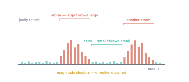
*Figure 1.* The absolute size of each day's return through time. Large moves arrive in bunches (the storms) and quiet days in long calm stretches. The **magnitude** clusters and is forecastable; the **direction** is not.

Homoskedasticity has to break

Everything so far leaned on a quiet assumption that now must fall: ordinary regression assumes homoskedasticity, a constant error variance — every residual drawn from the same fixed-width distribution. Returns laugh at this. Their variance breathes — large in the clusters, small in the calms. A model that pretends variance never changes is overconfident in storms and underconfident in calm: exactly backwards for sizing risk. (This is the ARCH signature you tested for in ch3; here we stop testing and start modelling.)

From ARCH to GARCH

The fix is to stop treating variance as a fixed number and start treating it as a process with its own memory. Robert Engle introduced it in 1982 (a 2003 Nobel), and his student Tim Bollerslev generalized it. Engle's ARCH(q) makes today's variance a weighted sum of recent squared shocks:

$\sigma_t^2 = \omega + \alpha_1 r_{t-1}^2 + \cdots + \alpha_q r_{t-q}^2.$

A big move yesterday raises today's variance — clustering, captured. But to reach far back you'd need many lags. Bollerslev's insight was to add one term that carries all of history recursively — yesterday's variance — giving the GARCH(1,1):

$\boxed{\ \sigma_t^2 = \omega + \alpha\,r_{t-1}^2 + \beta\,\sigma_{t-1}^2\ }$

Read it as a blend: today's variance is a constant floor $\omega$ , plus a fresh jolt from yesterday's squared return ( $\alpha\,r_{t-1}^2$ ), plus an inherited level from yesterday's variance ( $\beta\,\sigma_{t-1}^2$ ). One squared-return lag, one variance lag — the workhorse of the entire field.

The three numbers: ω, α, β

Three parameters run everything. $\omega$ is the floor — the baseline variance always present. $\alpha$ is the reaction: how sharply variance jumps after a fresh shock (large $\alpha$ = jumpy, snapping to attention after every big day). $\beta$ is the memory / persistence: how much of yesterday's variance survives into today (large $\beta$ = storms decay slowly, calm lingers).

Two conditions keep it sane. All three must be non-negative (variance can't go negative), and crucially $\alpha + \beta < 1$ . That sum is persistence — the closer to 1, the longer a shock echoes. Below 1 the process is stationary and pulled back toward a long-run (unconditional) variance:

$\bar\sigma^2 = \frac{\omega}{1 - \alpha - \beta}.$

This is the gravitational center the process orbits: after a shock, GARCH decays the variance back toward $\bar\sigma^2$ , and the speed is set by $\alpha+\beta$ — the shock's half-life is $\ln(0.5)/\ln(\alpha+\beta)$ . For daily equities $\alpha+\beta$ is famously near 1 (often above 0.95), so half-lives run to weeks — the mathematics restating what your eyes saw in ch4: volatility has long memory, it is stubbornly persistent.

An old friend: EWMA is GARCH without mean reversion

You have already met a cousin of this equation. Set $\omega = 0$ and $\alpha + \beta = 1$ (write $\alpha = 1-\lambda$ , $\beta = \lambda$ ) and GARCH collapses to

$\sigma_t^2 = (1-\lambda)\,r_{t-1}^2 + \lambda\,\sigma_{t-1}^2,$

which is exactly the EWMA / RiskMetrics estimator from Module 102-5. So the EWMA you built there is a special integrated GARCH (IGARCH) — GARCH with the persistence pinned to 1 and no long-run level to revert to. That's its one weakness: it tracks volatility responsively but, lacking mean reversion, its long-horizon forecast never comes home. Full GARCH restores the missing floor. The loop from 102 closes here.

How the parameters are found: maximum likelihood

Where do $\omega, \alpha, \beta$ come from? Maximum likelihood — the engine of 201 ch1. Assume each return is conditionally normal with the time-varying variance the recursion produces, $r_t \mid \text{past} \sim \mathcal{N}(0, \sigma_t^2)$ , write the likelihood of the whole series, and climb it to its peak. (When returns are fatter-tailed than normal — they are — the same procedure run anyway is quasi-MLE, still consistent.) This is how SVQ, and every risk desk, turns a return history into a fitted $(\omega, \alpha, \beta)$ .

Forecasting: the volatility term structure

A fitted GARCH doesn't just describe today's variance — it forecasts tomorrow's, and the day after, and the whole path. The $k$ -step-ahead variance forecast mean-reverts geometrically to the long-run level:

$\mathbb{E}[\sigma_{t+k}^2] = \bar\sigma^2 + (\alpha+\beta)^{k-1}\big(\sigma_{t+1}^2 - \bar\sigma^2\big).$

If today's vol is above $\bar\sigma$ , the forecast decays down toward it; if compressed below, it drifts up. That curve of forecasts across horizons is the volatility term structure.

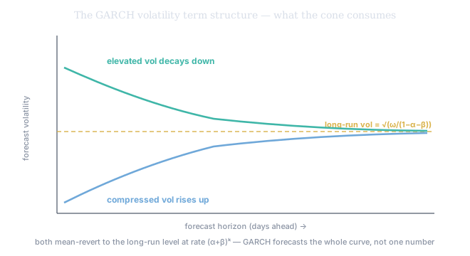
*Figure 2.* GARCH forecasts the whole curve, not one number. From an elevated start the forecast decays toward the long-run level; from a compressed start it rises toward it — both mean-reverting at rate $(\alpha+\beta)^k$. This is the term structure that upgrades the probability cone: the cone of Module 102-2, drawn with a *constant* σ and flaring like √t, becomes a GARCH cone whose flare *itself* changes with the vol regime — wide-but-settling after a storm, narrow-but-widening in a squeeze. — *Figure 2.* GARCH forecasts the whole curve, not one number. From an elevated start the forecast decays toward the long-run level; from a compressed start it rises toward it — both mean-reverting at rate $(\alpha+\beta)^k$ . This is the term structure that upgrades the probability cone: the cone of Module 102-2, drawn with a *constant* σ and flaring like √t, becomes a GARCH cone whose flare *itself* changes with the vol regime — wide-but-settling after a storm, narrow-but-widening in a squeeze.

The leverage effect

One honest refinement. Plain GARCH treats a $-6\%$ day and a $+6\%$ day identically — both enter as $r_{t-1}^2$ . But equities show the leverage effect: a drop raises future volatility more than a rally of the same size. The GJR-GARCH and EGARCH variants add an asymmetry term that fires harder on negative shocks. This is the same asymmetry as the equity skew — the downward-sloping wing slope of Module 202-1 — seen in the time domain rather than across strikes. Direction reappears not in the return but in how the return shapes tomorrow's risk.

Application: SVQ's GARCH

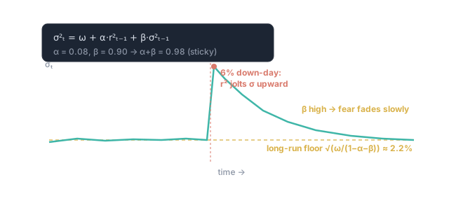
*Figure 3.* The recursion live: conditional vol hovers near its floor, a $6\%$ shock spikes the $\alpha$ term, and the forecast vaults up — then, because $\beta$ is high, that elevated fear bleeds off only slowly. The rising line is SVQ telling you the *magnitude* of further movement is now genuine evidence.

In Saqrid

SVQ's conditional-volatility panel is this recursion running live, $\sigma_t^2 = \omega + \alpha\,r_{t-1}^2 + \beta\,\sigma_{t-1}^2$ . Say the fit is $\omega = 0.00001$ , $\alpha = 0.08$ , $\beta = 0.90$ : then $\alpha+\beta = 0.98$ (high persistence, exactly what equities show), the long-run variance is $0.00001/(1-0.98) = 0.0005$ , and its square root is a daily-vol floor of about $2.2\%$ . A shock's half-life is $\ln(0.5)/\ln(0.98) \approx 34$ days. Now a $6\%$ down-day lands: its squared return $0.0036$ is more than seven times the long-run variance, so the $\alpha$ term injects a real jolt and tomorrow's forecast vaults up — and with $\beta = 0.90$ , that fear decays only slowly. The forecast panel carries the full term structure of Figure 2: how fast SVQ expects this storm to subside, which is exactly what the probability cone consumes to set its width at every horizon. And one parameter did the work: $\beta$ is why one bad day reshapes two weeks of expected risk.