Monte Carlo Simulation
Objectives
- Explain Monte Carlo as estimating an expectation by averaging simulations, justified by the law of large numbers, with error shrinking like 1/√N.
- Build a geometric Brownian motion path from drift and volatility, and use time-varying GARCH volatility for a regime-aware path.
- Run many paths and read the terminal cloud as a probability of profit, an expected value, and a tail risk (CVaR).
- Explain why simulation is necessary when no closed-form answer exists, and read a SVQ Monte-Carlo forecast.
You can now estimate two numbers from a return series — a drift and a volatility — and, from ch5, a volatility that changes over time. This final chapter of Tier 200 answers what to do with them. A drift and a volatility describe the engine; they don't tell you where the car ends up. To get from engine to destination you have to let it run — and since the future is uncertain, you don't run it once. You run it thousands of times and watch where it tends to go. That is Monte Carlo simulation, and it is the tool that ties this entire tier together.
Averaging simulations estimates an expectation
Beneath the casino imagery is one precise idea. Suppose you want a quantity that is really an average over an uncertain future — the expected payoff of a trade, the probability of clearing a target, the size of a bad-case loss. Formally each is an expectation for some function of a random outcome . When you can't evaluate that expectation with a formula, you estimate it: draw independent simulations and average,
Why is that legitimate? The law of large numbers (Tier 100 ch4): the sample average converges to the true expectation as grows. And the error obeys the rule you already know — the Monte Carlo standard error is , shrinking like . Remarkably, that rate does not depend on how many dimensions the problem has, which is exactly why simulation dominates once a problem gets complicated: a formula that would need a twenty-dimensional integral yields to the same dice.
The dice: pseudo-random shocks
Start with the dice. When your computer draws a "random" number it runs a deterministic recipe producing values so evenly spread and pattern-free that they behave like chance — pseudo-random numbers. The base ingredient is a draw from the uniform distribution on , and from it you can manufacture almost any distribution. The one finance wants is the normal: a standard-normal draw , mostly landing in , rarely beyond . That single number — a shock, or innovation — is the random heartbeat of every path.
Building a path
Put the shock to work with geometric Brownian motion (Module 102-2): over a small step , the log-price moves by a deterministic drift plus a random kick scaled by volatility:
(The is the volatility-drag correction from ch2 that keeps the average simulated price honest after exponentiating.) Chain the steps — twenty of them for a twenty-day horizon — each with a fresh shock, and you have drawn one complete path: one possible future, part determined, part luck.
Here is the ch5 upgrade that matters. Nothing forces to be constant. Feed each step the GARCH conditional volatility — updated by the recursion after every simulated move — and your paths breathe exactly as real volatility does: wide steps in the storm, narrow in the calm. A constant-vol simulation gives the tidy cone of ch2; a GARCH simulation gives the regime-aware cone, wide-but-settling after a shock, narrow-but-widening in a squeeze.
Many paths → the fan
One path tells you almost nothing — it could have been lucky. But run the construction five thousand times, each with its own independent shocks, and you get five thousand possible futures.
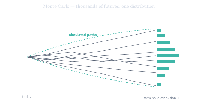
Figure 1. Paths spread from today into a fan; the envelope is the percentile cone (Module 102-2, now generated rather than assumed), and the histogram on the right edge is the distribution of ending prices. The middle of the cloud is your central forecast; its width is your uncertainty. This is the probability tunnel — Monte Carlo is what draws it.
Reading the cloud: POP, EV, and CVaR
The payoff of holding a distribution instead of a point is that you can now count and average anything. Three readings matter most, and they are exactly what turns a forecast into a trade decision:
- Probability of profit (POP) — the fraction of paths that finished past your target. Eight hundred of five thousand cleared the line? A 16% probability, read straight off the simulation.
- Expected value (EV) — the average payoff across all paths: your edge, if you have one.
- Conditional Value-at-Risk (CVaR) — the average of the worst outcomes (say the worst 5%): what a bad day actually costs you.
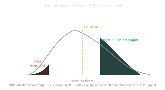
Figure 2. The simulated terminal cloud, read three ways: POP is the area past the target, EV is the mean, and CVaR is the average of the far-left tail. A trade can have a high POP and a positive EV yet a brutal CVaR — the short-volatility profile of 201 ch4 — which is why all three, not just the headline probability, decide whether to put it on.
This is the exact output that feeds SVQ's TEP Engine when it ranks trade ideas: POP, EV, and a CVaR-based size, all computed from a simulated cloud like this one.
How many paths? Convergence and variance reduction
Because the error is , quadrupling the paths only halves the error — precision is expensive, and beyond a point more paths barely move the answer.
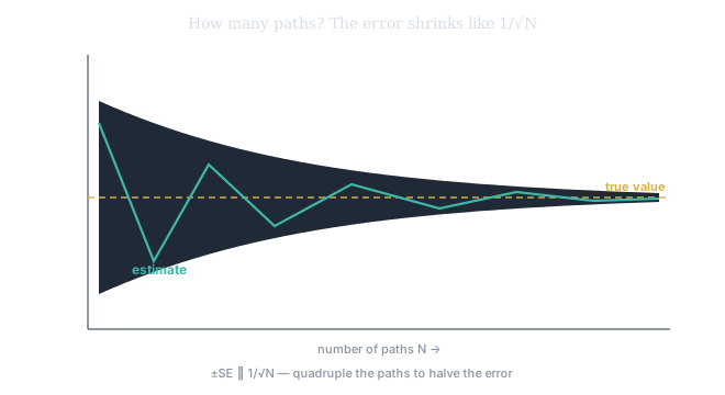
Figure 3. The estimate lurches at small and settles onto the truth as paths accumulate, inside a funnel that narrows like . This is why re-running a SVQ forecast with 1,000 vs 10,000 paths shifts the "probability above target" a little at first and then hardly at all: you've entered the flat part of the curve.
When you need more accuracy per path, variance reduction helps: antithetic variates (pair each shock with its mirror so lucky and unlucky draws cancel) and control variates (subtract off a related quantity you know exactly) can shrink without more paths. They buy precision with cleverness instead of compute.
Why simulate at all?
If GBM had a formula, why simulate? Because most real problems don't. Path-dependent payoffs — barriers that knock out mid-path, Asian options on the average price — depend on the whole journey, not just the endpoint, so no endpoint formula exists. Nonlinear dynamics like GARCH have no closed-form multi-step forecast at all (a fact from Tsay's forecasting chapter) — the only honest way to project a GARCH world forward is to simulate it. Fat tails, several correlated assets, early exercise: when the math has no closed form, you roll the dice. Simulation is the universal solvent of quantitative finance.
The Tier-200 capstone
Notice what this chapter gathered. The GBM of 102-2 supplies the step; the GARCH of ch5 supplies the breathing volatility; the law of large numbers of 101-4 makes the average trustworthy and the 1/√N of 101-5 tells you how many paths; the cone of 102-2 is the picture; and POP/EV/CVaR of 201-4 are the decisions. Monte Carlo is where the whole intermediate tier converges into one working engine — and it is the natural doorway to Tier 300, where continuous-time stochastic calculus gives these paths their rigorous foundation.
The SVQ forecast panel is a Monte Carlo engine wearing a chart. It pulls the asset's drift and (GARCH) volatility from recent returns, simulates a few thousand paths forward over your horizon, and draws them: the faint fan is the raw paths, the shaded cone is the percentile band. When it prints "62% chance above 4,500 in 20 sessions," it counted the fraction of paths that finished above 4,500 — POP, exactly as you learned. Further down it reports the EV and a CVaR-based position size from the same cloud. A wider volatility input flares the cone and drifts that probability toward fifty-fifty: more uncertainty, and the target stops being evidence of anything.