Time Series: Stationarity, AR & MA
Objectives
- Define weak stationarity and connect non-stationary prices to a unit root — the random walk is an AR(1) with φ = 1.
- Compute and read an autocorrelation function against its noise band, and tell genuine persistence from chance.
- Write AR(p) and MA(q) processes, distinguish them by their ACF/PACF signatures, and not confuse the MA process with the moving-average smoother.
- Explain mean reversion and long memory, and write the HAR decomposition of realized volatility into daily, weekly, and monthly bands.
Up to now you have treated your observations as a bag of independent draws — each return sampled fresh, yesterday telling you nothing about today. That assumption made the last three chapters' regression machinery run cleanly. It is also, for almost every financial series you will touch, false. A time series is a sequence where order matters: today's value is entangled with yesterday's, last week's, sometimes last month's. The whole job of time-series analysis is to measure that entanglement honestly — to separate the part of today that was genuinely predictable from the part that was new. It is the same question the institute keeps circling: when is a number real evidence, and when is it just the past echoing forward and fooling you?
Stationarity, the foundation
Before you can measure persistence, you need a foundation stable enough to stand on: stationarity. A series is weakly stationary when three things hold steady over time:
The mean doesn't drift, the variance doesn't balloon, and the relationship between a value and one a fixed distance behind depends only on that distance — not on where in the calendar you stand. A stationary series has no preferred moment; a January window looks statistically like an August one. This matters because nearly every estimator you own — a mean, a variance, a correlation — silently assumes the thing you're averaging keeps its identity across the sample. Average a series whose mean is wandering and you get a number that describes nowhere.
Raw prices are the classic offender, and now we can say precisely why. A price behaves like a random walk, — and that is exactly an AR(1) with coefficient one, a unit root. With the coefficient at one, shocks never fade; they accumulate forever, so the mean wanders and the variance grows without bound. (This is the same random walk from Tier 100 ch4, now named formally.) The augmented Dickey–Fuller test checks for that unit root, and the fix is differencing: subtract consecutive prices and you get returns, which are close to stationary. That is not an aesthetic choice — it is what makes the rest of this lesson legitimate.
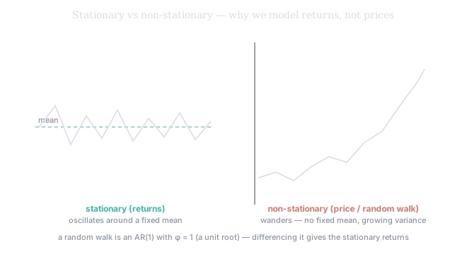
Figure 1. Two series. The stationary one (left) oscillates around a fixed mean, forever returning to it — a January stretch looks like an August one. The random walk (right) wanders off with no fixed mean and swelling spread. Differencing the walk (price → returns) collapses it to something like the left panel — which is why we model returns.
The autocorrelation function
To measure how a series remembers its own past, compute its autocorrelation. Lay a copy of the series beside itself shifted by steps, correlate the two columns, and you have the autocorrelation at lag :
The division normalizes every reading to so you can compare lags fairly. Do it for every lag and you trace the autocorrelation function (ACF). But a sample ACF is never exactly zero even on pure noise, so the guardrail is a band of roughly : a bar inside it is noise in a costume; a bar poking clearly outside is genuine memory. Same discipline as a regression t-statistic, transplanted into time.
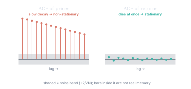
Figure 2. The ACF of raw prices (left) decays so slowly that nearly every lag pokes far above the band — the series remembers its whole past, the signature of non-stationarity. The ACF of returns (right) collapses inside the band immediately: yesterday's return barely predicts today's.
Two engines: AR and MA
With the ACF in hand, name the two elementary engines. The autoregressive process (AR) says today is a fraction of its own past plus a fresh shock:
For the simplest, AR(1), is stationary if and only if — and then it is mean-reverting: after a shock, the series is pulled gradually back toward its mean, with a shock's half-life of . That is the formal engine behind ch1's "regression toward the mean," and it is why an extreme volatility reading tends to revert (the squeeze you met in 201). Push to 1 and reversion vanishes — the random walk again. The AR fingerprint is an ACF that tails off smoothly, because yesterday already contained a piece of the day before, so any shock decays gradually.
The moving-average process (MA) builds today out of recent shocks:
Here memory is finite and blunt: an MA(1) knows exactly one step back and nothing beyond, so its ACF cuts off sharply — a spike, then silence. (A word of caution: this MA process is not the moving-average smoother of 102 ch5. There, a moving average was a filter you slid over the observed series to smooth it; here, it is a model that builds the series out of unobserved past shocks. Same two words, entirely different object — context tells you which.) Combine the two and you get an ARMA model.
The identification mirror: ACF and PACF
To tell AR from MA cleanly, bring in the ACF's partner, the partial autocorrelation function (PACF), which measures the lag- correlation after stripping out everything the shorter lags already explained. The classic signature: an AR process cuts off in the PACF and tails off in the ACF; an MA process does the reverse. That mirror is the workhorse of model identification (Box–Jenkins).
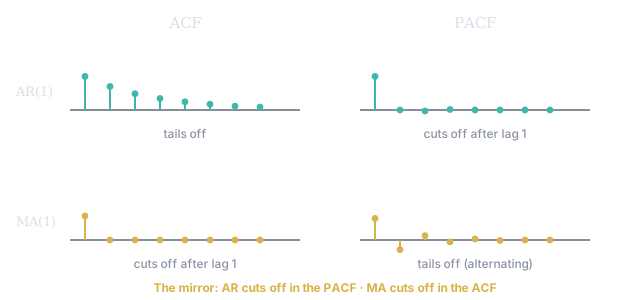
Figure 3. The identification mirror. An AR(1) (top) tails off in the ACF but cuts off after one lag in the PACF. An MA(1) (bottom) does the exact reverse. Read the two plots together and the process names itself.
Long memory and the HAR model
One more fact, and it is where volatility forces our hand. The ACF of realized volatility does not tail off in a handful of lags like a well-behaved AR(1) — it decays slowly, over dozens of lags, a property called long memory. Volatility is sticky: today's reading remembers weeks of its own past (the clustering you first saw in Tier 100 ch2, now measured). A single AR(1) can't capture that — its memory fades too fast — and fitting a 22-lag AR means 22 noisy coefficients.
The elegant shortcut is the HAR model (Heterogeneous AutoRegressive). Instead of 22 separate lags, pool them into three economically meaningful bands — the last day, the last week (5-day average), and the last month (22-day average):
Three coefficients capture the long memory that would otherwise take twenty. The name's "heterogeneous" is the reason it works: markets are made of participants acting on different horizons — day traders, swing traders on weekly rhythms, institutions on monthly ones — and each imprints its own layer of persistence. HAR gives each layer its own coefficient.
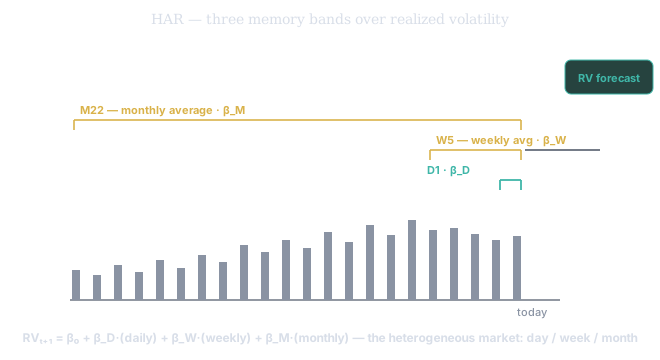
Figure 4. HAR as three nested memory bands over the realized-vol series: the daily term (), the 5-day weekly average (), and the 22-day monthly average (), combining into tomorrow's forecast. Long memory, captured by three coefficients instead of twenty-two.
SVQ's HAR decomposition is this lesson made concrete: today's realized volatility modelled as a weighted sum over the daily, weekly-5, and monthly-22 horizons — structurally an autoregression on volatility with three memory bands stacked. It works because of the exact autocorrelation you just studied: the RV ACF tails off slowly over dozens of lags, so pooling lags into daily/weekly/monthly buckets captures that long memory cheaply. When SVQ shows the three component loadings (, , ), you are reading how much of tomorrow's expected volatility is genuine evidence from yesterday versus the slower weekly and monthly tides. And when even HAR's residuals still cluster in variance, you've reached the next chapter's tool — a full GARCH model of the volatility itself.