Diagnostics: Heteroskedasticity & Autocorrelation
Objectives
- Read residuals as the window into the OLS assumptions, and explain why heteroskedasticity and autocorrelation leave the slope unbiased but make its standard errors wrong.
- Diagnose both from residual plots and the residual ACF, and name the formal tests (Breusch–Pagan/White; Ljung–Box, Durbin–Watson/Breusch–Godfrey).
- Run the ARCH test on squared residuals and recognize it as the signature that calls for a GARCH model.
- Repair inference with White or Newey–West (HAC) standard errors — or by modelling the variance — rather than re-estimating the slope.
A regression can be right about the slope and lying to you about everything else.
That sentence is the whole chapter. When you fit OLS you get two things: coefficients (the slopes) and standard errors (how much to trust them). The last two chapters taught you to read the slope; here you learn that the second number rests on assumptions about the residuals — the leftover errors the model couldn't explain — and that when those assumptions break, the slope can stay perfectly fine while the standard error becomes fiction. Since every t-statistic and p-value is the slope divided by its standard error, a corrupted standard error corrupts your verdict on whether a number is genuine evidence. You can be confident about a relationship the data does not support.
Interrogate the residuals
You never observe the true errors , but you observe the residuals — your estimates of them:
The residuals are the diagnostic surface. Plot them, correlate them, test them — every assumption from ch1 and ch2 leaves its fingerprint here. Two failures dominate finance, and you will see both constantly.
Heteroskedasticity
OLS assumes the residuals all share one variance — the model is wrong by roughly the same amount everywhere. That is homoskedasticity, , constant. Heteroskedasticity is when the scatter is not equal, — tiny in some regions, large in others. The signature is a residual plot that fans out like a megaphone: tight on one side, spreading wide on the other.
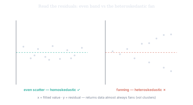
Figure 1. Residuals against fitted values. On the left, an even random band — homoskedastic, healthy. On the right, the megaphone fan — the variance grows with the fitted value. Returns data almost always looks like the right panel.
And finance is heteroskedasticity's natural home, for a reason you've known since Tier 100: volatility clusters. Markets go through quiet stretches where a model fits snugly, then erupt into turbulence where the same model misses by enormous margins. The residual variance is not constant — it tracks the volatility regime. So if your dependent variable touches returns or volatility, you should expect heteroskedasticity, not be surprised by it.
Autocorrelation
OLS also assumes the residuals are independent — that today's error tells you nothing about tomorrow's. In a time series that is heroic. If the model under-predicts today, it often under-predicts tomorrow too, because the thing it's missing persists; errors come in runs. The cleanest diagnostic is the autocorrelation function (ACF) of the residuals: the correlation of the residual series with its own past, lag by lag, with a band marking "indistinguishable from zero."
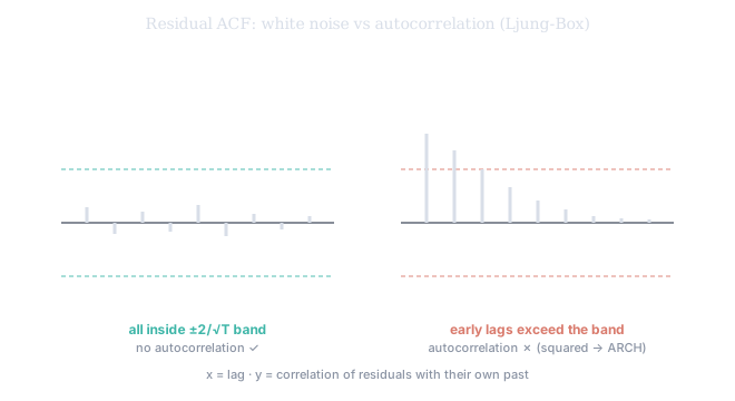
Figure 2. Residual ACF. White-noise residuals (left) keep every bar inside the band. Autocorrelated residuals (right) poke above it at the early lags and decay slowly — the model is leaving predictable structure on the table. (Run the same ACF on the squared residuals and persistent bars there mean clustered variance — the ARCH signature below.)
To put a number on it, the Ljung–Box portmanteau test asks whether the first autocorrelations are jointly zero:
and a large (small p) rejects "no autocorrelation." The classic one-lag shortcut is the Durbin–Watson statistic, , running 0–4: near 2 is clean, near 0 is strong positive autocorrelation, near 4 is negative. Durbin–Watson sees only lag 1; Breusch–Godfrey and Ljung–Box check many lags at once.
Neither biases the slope — both wreck the standard error
Here is the most misunderstood point in applied regression, so hold onto it. Neither pathology biases the slope. Heteroskedasticity and autocorrelation do not push your coefficient toward the wrong value; on average it still lands in the right place. What they wreck is the precision — the standard error. In the cases that dominate finance — positive autocorrelation and volatility-clustered heteroskedasticity — they make OLS report standard errors that are too small, t-statistics too large, and significance where none exists. (The bias can run the other way — negative autocorrelation makes tests too conservative — but the dangerous, common direction manufactures false significance.)
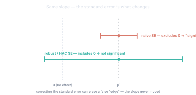
Figure 3. The same slope, two intervals. The naive standard error gives a too-narrow interval that excludes zero — a confident "significant." The robust interval, computed honestly, is wider and includes zero — not significant. The slope never moved; only the truth about its uncertainty did. This is why "fixing" the problem by re-estimating the slope is exactly backwards.
The formal tests
To diagnose heteroskedasticity, the workhorses are Breusch–Pagan and White's test: regress the squared residuals on the predictors; if the variance has no pattern, that regression explains nothing and the test is quiet; if the squared residuals grow with a regressor, it fires. White's is more general (it adds squares and cross-products).
And one test bridges directly into the next chapter. Apply the Ljung–Box test to the squared residuals and you get the ARCH test (Engle's): persistent autocorrelation in means the variance itself is autocorrelated — calm follows calm, storms follow storms. That is not noise to be robust-against; it is structure to be modelled, and the model that captures it is GARCH, the subject of ch5. The ARCH test is how you know you've outgrown robust standard errors and need a variance model.
Two more checks: normality and influence
Two quick diagnostics complete the kit. A QQ-plot of the residuals (Tier 100 ch2) checks the normality assumption that exact small-sample inference rests on — residuals bending off the line at the tails warn that your p-values are approximate. And leverage / influence measures (Cook's distance) flag the single points doing outsized work: one extreme observation can swing a whole fit, and you should know whether your "relationship" is real or the puppetry of one outlier.
The repairs
Once diagnosed, repair the standard error — not the slope. For heteroskedasticity, use heteroskedasticity-robust (White / Huber–White, "HC") standard errors. For autocorrelation — usually alongside heteroskedasticity — use Newey–West HAC standard errors (heteroskedasticity- and autocorrelation-consistent). These leave the coefficients untouched and simply tell the truth about trust. The more ambitious route is to model the changing variance directly — exactly what GARCH does, where this course heads next.
SVQ's regression-diagnostics panel plots the residuals of a returns series. The residuals from a returns model almost never show the calm, even band of homoskedasticity — the scatter bunches around the volatile periods, widening exactly where realized vol spiked and narrowing through the quiet. That is heteroskedasticity in returns made visible, and it is the structural reason SVQ defaults to robust / HAC standard errors on return-based fits — the very correction behind the significance flags you met on the VRP and wing-slope tests. When the panel flags a relationship as significant, it has already corrected for this fanning, so the green light means genuine evidence. And when the squared residuals show ARCH, SVQ stops correcting and starts modelling — the GARCH handoff of the next chapter.