Multiple Regression & Its Assumptions
Objectives
- Write the multiple-regression model in matrix form and compute the OLS estimator β̂ = (XᵀX)⁻¹XᵀY.
- Interpret each coefficient as a partial effect — the move in y per unit of one predictor, holding the others fixed — and recognize omitted-variable bias.
- Quantify multicollinearity with the variance inflation factor, and use adjusted R² and the overfitting tradeoff to decide how many predictors to keep.
- State the five classical assumptions and what breaks when each fails, and use an F-test for joint significance.
- Reframe a raw two-point wing slope as a level-controlled multiple regression on the crash-o-meter.
In the last chapter you fit a line to one predictor: a single slope, a single intercept, a cloud of points. That model answered one question — as moves, how does tend to move with it? A good question. But the world rarely hands you one predictor at a time, and when you force a one-variable line onto a many-variable reality, the slope you get back can lie to you in a very specific way. This chapter is about adding predictors — not because more is better (it usually isn't), but because the move from one to several changes what a slope means.
The confounding problem
Suppose you want to know how steeply implied vol rises as you walk into the deep tail of a smile. You could draw a line through two points — the near wing and the far wing — and read its slope. A perfectly good single-variable answer. But the tail's steepness is not the only thing moving: the overall level of volatility drifts up and down, and the smile gets more or less curved. Measure tail steepness with one crude slope on a day when the entire surface has lifted, and you cannot tell whether the tail is genuinely more fearful or whether everything simply got more expensive at once. The single number has confounded two stories. Multiple regression pulls them apart.
The model and the matrix form
In multiple regression you model as a linear combination of several predictors plus noise:
Stack all observations and it collapses to one clean matrix equation,
where is the column of outcomes, is the design matrix (one row per observation, one column per predictor, plus a leading column of ones for the intercept), and is the vector of coefficients. We estimate it the same way as before — minimize the squared residuals — and the solution has a closed form worth committing to memory:
Read it slowly. is a small square matrix capturing how the predictors covary with each other; inverting it is precisely the step that de-correlates them, so each coefficient reflects its own contribution and not its neighbour's. That inversion is the mathematical machinery of "holding the others fixed."
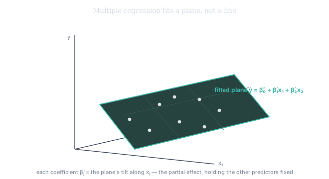
Figure 1. With two predictors, OLS fits a plane through a 3-D scatter (with more, a hyperplane you can't picture but the algebra handles identically). Each coefficient is the plane's tilt along one axis — how changes as moves and the other predictors are held fixed.
The partial effect
Here is the sentence that matters most in the chapter: each slope is the expected change in for a one-unit increase in , holding every other predictor fixed. That phrase — holding the others fixed — is what a single-variable regression cannot give you, and it is exactly what cures the confounding problem. is a partial effect: the steepness of the tail after the overall level has been accounted for.
The five assumptions — and omitted-variable bias
The formula always returns an answer. Whether it means anything rests on five classical assumptions a serious analyst can recite:
- Linearity — really is a linear function of the predictors plus noise.
- No perfect multicollinearity — no predictor is an exact linear combination of the others; if two columns of carry the same information, cannot be inverted.
- Exogeneity — ; the errors are uncorrelated with the predictors.
- Homoskedasticity — the error variance is constant across observations.
- No autocorrelation — the errors are uncorrelated with each other (the one that bites hardest in time series — the bridge to the rest of this course).
The first three buy you unbiased coefficients; the last two buy you trustworthy standard errors. The exogeneity failure has a name you met in Tier 100 ch6: omitted-variable bias. If you leave out a variable that affects and is correlated with an included predictor, that predictor's coefficient absorbs the missing effect and becomes biased — it is no longer a clean partial effect but a confounded one. A steep, impressive slope estimated on data that violates exogeneity is not evidence of anything except your own optimism.
Multicollinearity, quantified
"No perfect multicollinearity" is the hard requirement; near multicollinearity is the practical menace. When two predictors are highly correlated, is nearly singular and its inverse blows up — so the coefficient standard errors balloon. The diagnostic is the variance inflation factor: regress predictor on all the others, get its , and
As (predictor is well-explained by the others), and that coefficient's variance explodes. The symptom: coefficients that are individually insignificant, wildly unstable, and prone to flip sign when you nudge the data — because the regression genuinely cannot separate two predictors that move together. (Note: collinearity damages the individual coefficients, not necessarily the model's predictions.)
More isn't better: adjusted R² and overfitting
Why not just throw in every predictor you can find? Because R² can only rise when you add a predictor — even a column of pure noise. In-sample fit is a downward-biased, optimistic measure of real performance: the model can always contort itself to hug the data it was fit on. This is the bias-variance tradeoff (Tier 100 ch5) in model-selection clothing: too few predictors underfits (high bias, missing real structure); too many overfits (high variance, fitting noise that won't repeat), and it is the very backtest illusion of ch6 — spectacular in-sample, useless out-of-sample.
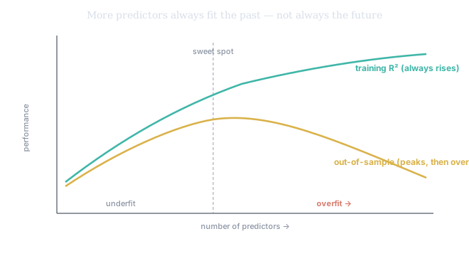
Figure 2. Add predictors and the training R² climbs forever (teal). But out-of-sample performance (gold) rises, peaks, then falls as the extra predictors start fitting noise. The sweet spot is the peak — and finding it is the whole game of model selection.
The honest fix is to penalize complexity. The simplest is adjusted R², which docks the fit for each predictor used:
so it rises only if a new predictor earns its keep against the degrees of freedom it costs. More principled criteria — Mallows' , AIC, BIC, and cross-validation — formalize the same instinct: reward fit, punish complexity, and aim for the model that will predict, not just the one that flatters the past.
The F-test: are the predictors jointly useful?
The individual t-tests ask, one at a time, "is this coefficient nonzero?" The F-test asks a different, joint question: "taken together, do these predictors explain better than the intercept alone?" This matters precisely under collinearity, where each coefficient's t can look insignificant (their effects can't be cleanly separated) even though the group is jointly, decisively significant. Read the F first for "is there anything here at all," then the t's for "which pieces."
Application: the crash-o-meter
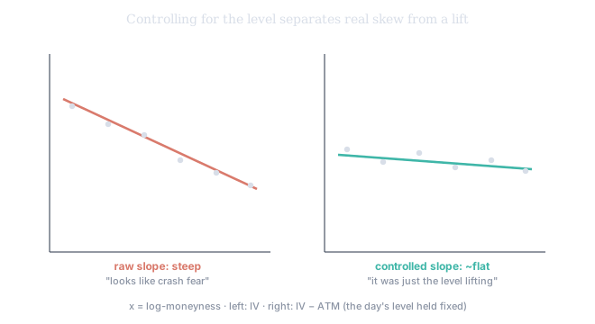
Figure 3. The raw smile (left) looks steep — apparent crash fear. Subtract the day's ATM level from each wing (right) and the slope nearly vanishes: the steepness was just the whole surface lifting. The partial effect — log-moneyness slope holding the level fixed — is the honest measure of tail fear.
The SVQ Crash-O-Meter shows a per-wing slope readout. Today's two-point put-wing slope is the change in IV from the 25-delta put to the 5-delta put, divided by the absolute log-moneyness between them — a clean rise-over-run on two anchors. That single-variable slope works, but it has a blind spot: on a day when the entire surface lifts, the raw slope rises even if the tail's relative fear is unchanged. The institute-grade upgrade is a multiple regression — and its design takes care, because a single day's three put anchors cannot identify it. With only three rows, the ATM level is one scalar pinned to all three, so its column is constant and perfectly collinear with the intercept (the exact multicollinearity violation above), and three parameters on three observations leaves zero residual degrees of freedom — no standard errors. The fix is pooling across days: many days of the 5-, 10-, and 25-delta put anchors stacked into one panel — each (day, anchor) pair an observation, the response that anchor's IV, the predictors log-moneyness and that day's ATM level (which now genuinely varies down the column). With dozens of days there are ample residual degrees of freedom, and the log-moneyness coefficient is the wing slope holding the overall vol level fixed — pure tail steepness. When that controlled coefficient is large with a small standard error, crash protection is genuinely being bid; when the raw slope is large but the controlled one collapses, the "fear" was just the surface repricing. (The one-day shortcut is IV-minus-ATM against log-moneyness — ATM as its own regressor on a three-point within-day sample is never identified.)