Simple Linear Regression (OLS)
Objectives
- Fit a simple linear regression by ordinary least squares and interpret the slope and intercept in the units of the problem.
- Recognize the slope as the covariance over the variance, and the fitted line as the estimated conditional expectation E[Y|X].
- Compute and interpret R² as the fraction of variance the regression explains.
- Get the standard error of the slope, turn it into a t-statistic and confidence interval, and know that least squares is maximum likelihood under normal errors.
- Read SVQ's wing slope as a regression of implied vol on log-moneyness, and judge whether the skew is real or noise.
You already know how to draw a line through a cloud of points. This chapter answers the harder, more useful question: which line exactly, how much should you believe its slope — and why regression turns out to be the same conditional expectation and covariance you've been building since Tier 100.
The model
You have paired observations: for each point an input and an output , and you suspect moves with in a roughly straight-line way. The honest model is a line plus noise:
is the intercept (where the line crosses the vertical axis), is the slope — the thing you actually care about, because it says how much changes per one-unit change in . The error is your admission that the world is not a perfect line. That scatter is not your enemy; it is the very thing that lets you ask whether the slope you found is real.
Ordinary least squares
For any candidate line, each point has a vertical gap to it — a residual. A good line makes the residuals small. Ordinary least squares (OLS) picks the unique line minimizing the sum of squared residuals:
We square for two reasons you've seen before (ch3 of Tier 100): squaring stops a big positive gap from cancelling a big negative one, and it punishes large misses far more than small ones, so the fit refuses to shrug off an outlier.
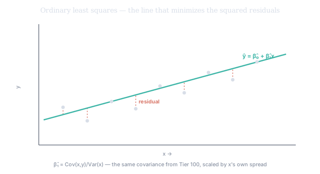
Figure 1. The fitted line and the vertical residuals. OLS is the single line for which the sum of the squared lengths of those red segments is as small as it can be. Every other line — flatter, steeper, shifted — makes that total larger.
The estimates — and an old friend
Grind through that minimization (it is worth seeing done by hand once) and two clean formulas drop out:
Read the slope slowly, because it is not a new object. It is the covariance of Tier 100 ch3 — how and move together — divided by the variance of — how moves on its own. Regression's slope is the covariance, rescaled by the input's own spread. The intercept then simply forces the line through the centre of mass: the fitted line always passes through .
And the line itself is an old friend too. In 102 ch3 you met the regression function — the best possible prediction of given . There it was an abstract conditional expectation; here OLS estimates it from data, under the working assumption that it is a straight line. So regression is not a new idea bolted on — it is conditional expectation made concrete and covariance turned into a testable slope. The whole statistical arc closes here.
How good is the fit? R²
A slope tells you the direction and strength of the relationship, but not how tightly the data follows it. For that we reach back, again, to 102 ch3 — the law of total variance, . The coefficient of determination is exactly the explained fraction:
where RSS is the residual sum of squares and TSS the total sum of squares of about its mean. An of 0.9 means the line accounts for 90% of 's variation and only 10% is residual scatter; an of 0.1 means the relationship, even if real, explains almost nothing.
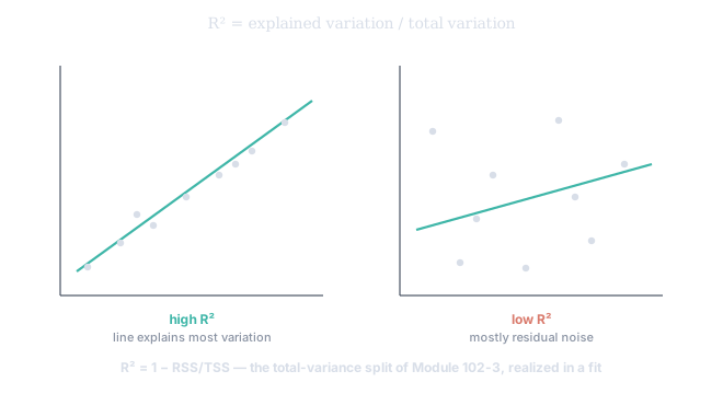
Figure 2. Same idea, two fits. On the left the points hug the line — high R², the regression explains most of the variation. On the right they scatter loosely around an identically-sloped line — low R², mostly residual noise. R² is the total-variance decomposition of Module 102-3, realized in an actual fit. (A warning for later: R² rewards adding variables even useless ones, which is why ch2 introduces the adjusted version.)
Least squares is maximum likelihood
Why squared residuals, and not, say, absolute ones? There's a deep answer from 201 ch1: if the errors are normally distributed, then minimizing the sum of squared residuals is exactly maximizing the likelihood. OLS is the maximum-likelihood estimator under Gaussian noise — not an arbitrary convention but the principled estimate when the scatter is bell-shaped. That also surfaces the assumptions OLS quietly rests on, and which you will learn to check in ch3: the relationship is genuinely linear, the errors have zero mean and constant variance, they are independent, and (for exact small-sample inference) roughly normal. As Wasserman puts it, the inferences are most trustworthy "when the residuals behave like random normal numbers." When they don't, the fit can still be computed — it just lies about its own certainty.
Is the slope real? Standard error, t, and CI
Here is what separates a quant from someone who merely owns a spreadsheet. Your estimate is almost never exactly zero, even when and are unrelated, because random scatter always conjures some accidental tilt. The whole discipline of inference (201) exists to ask: is this slope evidence, or noise that survived by luck? You need the standard error of the slope:
and staring at it tells you exactly when to trust a slope. The error shrinks — trust grows — when the residuals are small (points hug the line), when you have more data, and when the values are spread out (a wide lever arm pins the line down far better than a cramped cluster). Noisy data, few points, or bunched-up 's all inflate the error and tell you to hold your conclusion loosely.
Then inference is mechanical, exactly as in 201 ch3. The t-statistic is the slope over its own standard error, — the effect measured in units of its own uncertainty. A near 2 sits about two standard errors from zero, the rough line for 5% significance; equivalently the confidence interval is . If it comfortably excludes zero, you have evidence; if it straddles zero, the data is consistent with no relationship at all, and honesty demands you say so.
A bonus: regression toward the mean
The word "regression" is a historical accident worth keeping, because it names a real trap. Galton noticed that unusually tall fathers tend to have sons closer to average height — the fitted slope is less than one, so predictions are pulled toward the mean. The same thing governs markets: an extreme reading — a huge IV spike, an outlier return — tends to be followed by a more average one, not because of any restoring force, but because extremes are partly luck, and luck doesn't repeat. Mistake that statistical reversion for a tradeable signal (or for the failure of a strategy) and you will misread the most ordinary thing in data. Extremes regress; plan for it.
Application: the wing slope
SVQ reports a wing slope on every volatility smile. It computes it by regressing implied vol on log-moneyness across the listed strikes — implied vol is , log-moneyness is , and the fitted slope is the "wing slope" the panel reports, while the intercept (at zero moneyness) is the ATM implied vol. A steep negative slope is the familiar equity skew: out-of-the-money puts priced richer than calls. But the number alone is not the whole story; how the strikes scatter around the fit matters just as much. A handful of illiquid strikes with wide scatter inflates — the small-, large-residual case — and an impressive-looking slope may not be statistically distinguishable from a flat smile. The slope is the headline; its standard error is whether the headline is true. (This same regression, run across maturities, is the crash-o-meter input of the next chapter.)
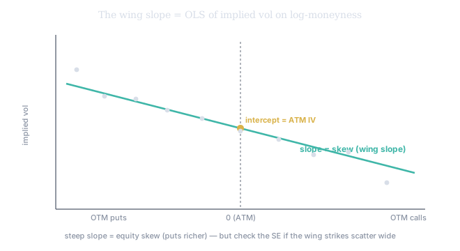
Figure 3. Implied vol against log-moneyness. The fitted line's downward slope is the skew (the wing slope); its value at zero moneyness is the ATM implied vol. When the wing strikes scatter wide, the standard error balloons and the skew may be inside the noise.