Hypothesis Testing: Significance, Errors & Power
Objectives
- Frame a trading question as a null and alternative hypothesis (one- or two-sided) and build a Wald/t test statistic.
- Interpret a p-value correctly and state what it is not; relate the significance level to the Type I error rate.
- Distinguish Type I from Type II error, define statistical power, and explain the three levers that raise it.
- Use the confidence-interval / test duality, and explain why statistical significance is not the same as effect size.
- Set up the implied-versus-realized volatility question as a one-sided paired test and read it as evidence, not proof.
Markets hand you suggestive numbers all day long. The hard part is never finding a pattern — it is deciding whether the pattern is real. Suppose that over the last sixty trading days, an option's implied volatility has sat consistently above what the underlying actually delivered. The implied vol looks rich; your instinct says sell it and collect the gap. But before you risk anything: is that gap genuine evidence that implied vol is overpriced, or the kind of gap that random noise throws up all the time? Hypothesis testing is the discipline that answers exactly that, and it is the spine of quantitative work.
The backwards move: null and alternative
The core move is strange at first. You do not try to prove what you believe. You set up the opposite and try to knock it down. The thing you try to knock down is the null hypothesis — always the boring, no-effect claim. Here, : on average, implied volatility equals realized; the gap is zero. The claim you care about is the alternative : implied vol is, on average, richer than realized. Formally you split the parameter into the null and alternative and write
Because points in one direction (richer, not merely different), this is a one-sided test — the right choice when you have a directional thesis. Had you only asked "is the gap nonzero?" you'd run a two-sided test (), the more common default. Why the backwards approach at all? Because it is far easier to rule something out than to prove it true. As Wasserman puts it, testing is like a legal trial: the null is presumed innocent, and you retain it unless the evidence strongly demands rejection.
The test statistic: the Wald test
To make "strongly demands" precise, build a test statistic — one number, computed from the data, that grows when the effect is real. Take each day's gap (implied − realized), average them, and scale that average by its own standard error. That is the Wald test (here a one-sample t-statistic):
which, under the null, behaves like a standard normal. It asks: how many standard errors above zero is the typical gap? A of 0.3 is a shrug; a of 3 is a thump on the table. We reject the null when lands in the rejection region , beyond a critical value chosen to control how often we're fooled.
The p-value, said correctly
Now the famous, frequently-mangled object. The p-value is the probability of a test statistic at least as extreme as the one you got, if the null were true:
Small means your data sit far out in the tail of the no-effect world — the boring story strains to explain them. You fix a threshold first, the significance level (often 0.05), and reject when .
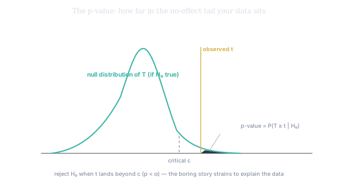
Figure 1. The distribution of the test statistic if were true. The critical value marks the rejection region; your observed lands beyond it, and the p-value is the shaded tail area past the observed value — the chance the no-effect world would produce data this extreme. Small tail, small p, reject.
Say this part out loud so you never get it wrong: the p-value is not the probability that the null is true, and not the chance you're wrong. It is the probability of your data under the null, nothing more. A p-value of 0.04 does not mean a 96% chance implied vol is rich — it means that in a world where implied and realized were truly equal, data this lopsided would appear about four times in a hundred. (This is the confusion-of-the-inverse from Tier 100 ch6: .)
Two ways to be wrong
Whenever you decide from a sample you can err in two distinct, asymmetric ways. A Type I error is rejecting a true null — you declared vol rich, sold it, but the gap was noise, and you bleed. Your significance level is this error rate: is the size of the test, , so choosing 0.05 means accepting being fooled one time in twenty. A Type II error is the opposite — failing to reject a false null: vol really was rich, the edge sat right there, and your test stayed silent. Its probability is .
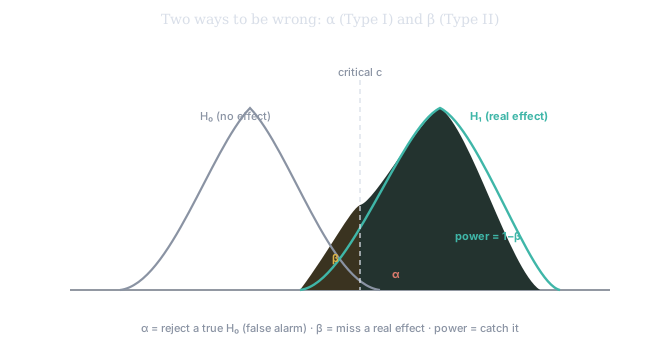
Figure 2. The two error types, drawn. The null (, gray) and the real-effect world (, teal) overlap, split by the critical value . The null's tail past is α (false alarm); the alternative's mass below is β (a missed real effect); everything to the right is power. Move to shrink one error and the other grows — the tradeoff is unavoidable.
Power: could you even have seen it?
This brings us to the quantity that separates a thoughtful analyst from someone who merely runs tests: power, — the probability the test detects a real effect when one exists. A low-power test is nearly worthless, because failing to reject then tells you nothing: you cannot distinguish "no edge" from "an edge I had no chance of seeing." Power climbs with three levers: a larger true effect, a smaller noise level, and — the one you usually control — a larger sample.
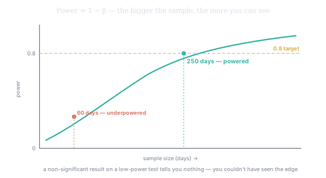
Figure 3. Power against sample size. With 60 days the test is underpowered — a real edge would clear the bar only sometimes — while at ~250 days the same edge reliably trips the test. This is why a non-significant result on a short window is not evidence of "no edge"; it is evidence you didn't look hard enough.
Two honest caveats
First, statistical significance is not effect size. With a huge sample the standard error shrinks toward zero, so even a microscopic, untradeable gap — a tenth of a vol point — produces a giant and a tiny p. "Significant" answers is it real?; it never answers is it big enough to matter after costs? Always read the magnitude, not just the verdict.
Second, a test and a confidence interval are two faces of one coin — the CI–test duality: rejecting at level is equivalent to falling outside the confidence interval from ch2. This is why Wasserman warns that you should often skip the test entirely and just report the interval: the interval shows the effect's size and uncertainty, while the test collapses all of that into a single reject/retain bit. Test when you have a sharp, pre-specified hypothesis; otherwise, let the interval speak.
Application: is implied vol richer than realized?
A name's daily implied- and realized-vol series over the last sixty sessions yields a daily gap, implied − realized. Its average — say +1.1 vol points — divided by the standard error of the gaps is the t-statistic. If that t-statistic comes out near 2.6 on 60 observations, the one-sided p-value lands near 0.005: under the null that vol is fairly priced, a tilt this rich appears less than once in a hundred such windows. That is a defensible reason to lean short volatility — and the start of next chapter's volatility risk premium. SVQ also quietly handles a subtlety: overlapping realized-vol windows make consecutive gaps autocorrelated, which shrinks the effective sample and inflates a naive t-statistic. The platform's significance flag corrects for that overlap — which is exactly why it sometimes refuses to light green on a gap the eye finds obvious.