Confidence Intervals & the Bootstrap
Objectives
- Construct and correctly interpret a confidence interval, stating what the confidence level does and does not promise.
- Define the empirical CDF and the plug-in principle, and see the bootstrap as plug-in applied to the sampling distribution.
- Explain why textbook standard-error formulas fail for realized volatility, and use the χ² exact interval to see why a variance CI is asymmetric.
- Build normal, pivotal, and percentile bootstrap confidence intervals, and choose the block bootstrap when returns are serially dependent.
- Read SVQ's 5/20/60-day realized-volatility windows through their bootstrap intervals to judge evidence versus noise.
Every number on a trading screen is an estimate wearing a disguise. When SVQ says an asset's realized volatility over the last twenty days is 24%, that looks like a fact. It is not — it is a single guess at a hidden truth, computed from a small, noisy sample of returns that happened to occur in one window. Rerun the universe, let a different twenty days unfold, and the same estimator prints something else. The honest question is never "what is the number" but "how much would it move if the world had dealt a slightly different hand." This chapter is about measuring that wobble — first with a formula, then, when the formula fails, by the most useful trick in modern statistics.
The confidence interval — and the misreading
Instead of a single point, report a confidence interval: a range plus a confidence level (90%, 95%) describing the procedure's long-run reliability. Hold onto the subtlety that trips up almost everyone: a 95% interval does not mean a 95% probability that the true volatility lies in this interval. The true value is fixed — it is either in or out. The 95% describes the method: repeat the whole estimation many times and about 95% of the intervals you build would cover the truth. You are buying a reliable procedure, not a probability about this one case. Treat the interval as your tool's batting average and you will never misread it.
The data is your estimate of the distribution
Before we build intervals, one foundational idea makes everything that follows — including the bootstrap — fall into place. You never see the true distribution that generates returns. But your sample is a picture of it, and we can make that precise. The empirical distribution function puts probability on each of your observations:
It is a staircase that steps up by at every data point, and a deep theorem (Glivenko-Cantelli) guarantees it converges to the true as the sample grows. That licenses the plug-in principle: any quantity you want is some functional of the distribution — the mean, the variance, volatility, a correlation, a quantile — and you estimate it by plugging in the empirical CDF, . Computing the sample volatility from your returns is the plug-in estimate of true volatility. Hold this idea; the bootstrap is nothing but plug-in applied one level up.
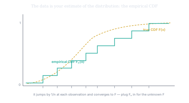
Figure 1. The empirical CDF (teal staircase) jumps by at each observation and hugs the smooth true CDF (gold). This is the formal sense in which "the data is your estimate of the distribution." Every statistic you compute is a feature of this staircase — and when you need the un-knowable true , you plug in instead.
Building the classical interval — and where it breaks
The classical recipe takes your estimate, finds its standard error, and steps out a couple of SEs each side: . For a sample mean this is beautiful, because the Central Limit Theorem hands you the standard error almost for free — — so a larger sample tightens the interval at the comforting rate of .
Now look at what SVQ actually computes, and the trouble appears. Realized volatility is not a mean. It is the square root of an average of squared returns — a nonlinear function built on second moments — and there is no clean textbook SE formula for it that survives contact with real markets. Returns have fat tails; volatility clusters, so today's squared return is correlated with yesterday's. The neat machinery quietly breaks, and any interval built from it is too narrow, too confident, and wrong in exactly the moments that matter.
Even in the idealized case it warns you about asymmetry. If returns were i.i.d. normal, the sample variance has an exact interval through the chi-squared distribution: , which gives
The χ² is skewed, so this interval is asymmetric — it reaches farther above the estimate than below — and for a 5-day window (, badly skewed) the asymmetry is severe. Volatility intervals lean upward, and that is not a quirk of any one method; it is the shape of variance estimation itself.
The bootstrap: plug-in by brute force
When the formula fails, resampling earns its place. The idea is almost insolent in its simplicity, and it is exactly the plug-in principle one level up. You wish you could draw many fresh samples from the true to see how your estimate varies — but you can't reach . So plug in : resample from your own data. Draw a new dataset of the same size by sampling your returns with replacement (the same return may appear twice or not at all), compute realized volatility on it, and repeat — a thousand or ten thousand times. You get not one number but a whole bootstrap distribution of plausible answers, and its spread is a remarkably good estimate of the real standard error — derived without writing down a single formula.
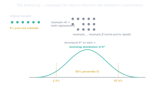
Figure 2. The loop. Resample the original sample with replacement many times (points repeat — that's the point), recompute the statistic on each, and the spread of those recomputed values is the bootstrap distribution. It is the sampling distribution you could never observe, simulated by plugging in for .
From that distribution you can read a confidence interval three ways. The normal interval uses the bootstrap's spread directly: . The pivotal interval works from the distribution of . The simplest and most popular is the percentile interval: sort your thousands of resampled volatilities and read off the values cutting the bottom and top 2.5% — those are the endpoints of your 95% interval. The bootstrap discovered the shape of the estimator's uncertainty by brute force — including its asymmetry — letting the data speak instead of forcing it through an assumption it violates.
The clustering trap and the block bootstrap
There is a trap here, and it is the same one that sank the formula. Drawing returns one at a time with replacement quietly assumes they are independent — that order doesn't matter. But volatility clustering means the opposite: violent days sit next to violent days. Resample single returns and you scatter the clusters, manufacturing a calmer, more independent world than the real one — so the plain bootstrap, like the formula, hands you intervals that are too narrow. The repair is the block bootstrap: resample contiguous blocks of returns — runs of five or ten consecutive days — and stitch them together. Each block carries its local stretch of clustering intact, so the dependence survives. Use the one-at-a-time bootstrap only when returns are near-independent; the moment serial dependence is in play — and in volatility it always is — resample in blocks.
Application: reading the realized-vol windows
SVQ shows three realized-volatility windows side by side. Suppose the 5-day reads 28%, the 20-day 24%, the 60-day 22%. The eye wants to call this a rising-volatility regime. Bootstrapping each window changes the story. The 5-day estimate, built on only five returns, comes back with a 95% interval running from roughly 15% to 41% — enormous, because with so few observations a single jumpy day dominates (and the χ² skew stretches it upward). The 60-day interval might be a tight 19% to 25%. Suddenly the picture changes: the 5-day "spike" sits comfortably inside the 60-day interval, so it is not yet evidence of anything. The shorter the window, the wider the interval, and the more skepticism a single reading deserves. The bootstrap is what reveals that, today, the headline number and the noise floor are the same height.
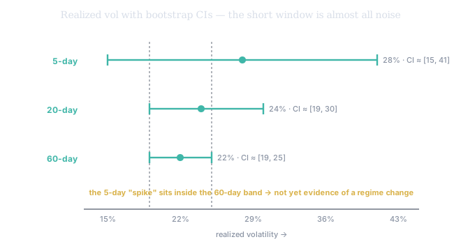
Figure 3. The three windows as point estimates with their bootstrap intervals. The 5-day bar is so wide it swallows the 20- and 60-day bars whole — its "spike" carries no information the longer windows don't already contain. Reading a volatility number without its interval is reading half the data.