Estimation: Sampling Distributions & Maximum Likelihood
Objectives
- State the three tasks of inference and explain why every estimate carries sampling uncertainty (the sampling distribution and standard error).
- Build an estimator by the method of moments and by maximum likelihood, and write the likelihood and log-likelihood.
- Explain why maximum likelihood is the default: consistency, asymptotic normality, and efficiency (the Cramér-Rao bound via Fisher information).
- Use the delta method to get the standard error of a transformed estimate, such as annualized volatility.
- Read SVQ's IV Rank, IV Percentile, and Z-score as 252-day estimates with their own sampling error, and recognize the vol models behind them as maximum-likelihood fits.
Welcome to the inference tier. Everything until now was preparation; here you learn the craft that defines quantitative finance — reasoning backward, from a finite sample of data to a statement about the unknown truth that produced it, with the uncertainty made explicit. Every inference problem is one of three tasks: point estimation (the single best value), confidence sets (an honest interval around it), and hypothesis testing (deciding whether an effect is real). This course teaches all three; this chapter is about the first, and about the one method — maximum likelihood — that builds nearly every estimate in modern finance.
Parameter, sample, and the sampling distribution
Start with the distinction the whole craft rests on. Imagine the true long-run behavior of an asset's volatility as a vast hidden urn containing every reading it could ever produce — the population. You never pour it out. You grab a handful — the last 252 trading days, say — and that handful is your sample. From it you compute a number (a mean, a percentile, a Z-score) and call it an estimate of the hidden parameter you actually want.
Here is the part that trips people up: grab a different year and you'd compute a different estimate, even though the underlying truth never changed. Your estimate wobbles from sample to sample. That wobble is not a bug — it is sampling, and because the estimate is itself random, it has its own distribution: the sampling distribution, the distribution of all the values your estimate could have taken. Its center, for a good estimator, sits on the truth (unbiased); its spread is the standard error — and the standard error, not the data's standard deviation, is what tells you how much to trust the number. For a sample mean,
which shrinks only as the square root of the sample size: to halve your uncertainty you must quadruple your data. (When you don't know σ — you almost never do — substitute the sample's own for the estimated standard error.) That much you met in Tier 100. Now the new question: where does an estimate come from in the first place?
Building an estimator
An estimator is a recipe that turns data into a guess. There are two classic ways to write one.
Method of moments
The simplest: match the sample to the theory. If a model says the population mean is some function of the parameter, set the sample mean equal to it and solve. Match as many moments as you have unknowns. The method of moments is quick and intuitive — but it is often not the best use of the data, which is why we reach for a sharper tool.
Maximum likelihood
The dominant method in all of statistics, and the engine under nearly every fitted model in finance, is maximum likelihood. Flip the usual question around. A density normally tells you how probable the data is for a fixed parameter. But you have the data — it's the parameter you don't know. So treat that same expression as a function of with the data fixed: the likelihood,
(We work with the log-likelihood because sums are easier than products and the maximum is in the same place.) The maximum-likelihood estimator (MLE) is the value that maximizes it — in plain words, the parameter value under which the data you actually observed is least surprising.
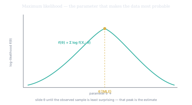
Figure 1. The log-likelihood as a function of the parameter. Each candidate assigns some probability to the sample you drew; the MLE is the peak — the that makes your observed data most probable. Estimation becomes an optimization: slide until the data is least surprising, and read off .
You have been doing this all along
Here is the reassuring punchline. Work out the MLE for a normal model and you find (the sample mean) and (the sample standard deviation). The estimators you have used since Tier 100 are maximum-likelihood estimators under the normal assumption — you just didn't know they had a pedigree. For a coin (Bernoulli), the MLE of the heads-probability is , the obvious fraction. Maximum likelihood agrees with common sense exactly where common sense is right.
Its power is where common sense runs out. Fitting a Student-t to returns to capture fat tails? The degrees-of-freedom parameter from Tier 100 ch2 is found by maximum likelihood. Fitting a GARCH model (next course) to capture volatility clustering? MLE. Calibrating an option volatility surface? A likelihood maximization. When SVQ characterizes a distribution or fits a volatility model, it is, under the hood, climbing a likelihood to its peak. This one idea is how essentially every model in finance meets the data.
Why maximum likelihood is the default
We prefer the MLE not by habit but because it is, in a precise sense, the best you can do. Three properties, all holding as the sample grows:
- Consistency — converges to the true as (it homes in on the truth).
- Asymptotic normality — . The MLE is approximately normal around the truth, which hands you a standard error and a confidence interval for free — the same machinery from Tier 100, now available for any model you fit.
- Efficiency — among well-behaved estimators, the MLE has the smallest possible variance. It attains the Cramér-Rao lower bound, a hard floor on how precise any unbiased estimator can be, set by the Fisher information — essentially how sharply peaked the likelihood is. A sharp peak means the data pin the parameter down tightly (much information, small SE); a flat peak means the data barely constrain it.
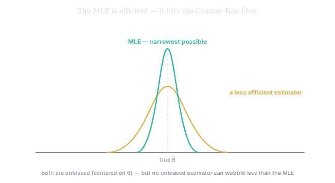
Figure 2. Two unbiased estimators of the same parameter, both centered on the truth. The MLE (teal) is the narrowest sampling distribution physically possible — it sits on the Cramér-Rao floor — while a less efficient estimator (gold) wobbles more for the same data. Efficiency is the prize: the MLE wrings the most precision out of every observation.
One more convenience, equivariance: the MLE of any function of θ is just that function of . If is the MLE of volatility, then is the MLE of variance — no re-derivation.
The delta method: error bars on transformed estimates
You rarely report a raw estimate; you transform it — daily volatility becomes annual, variance becomes standard deviation. How does the standard error travel through a transformation ? The delta method gives the answer with a one-line linearization:
Annualizing volatility is multiplication by , so its standard error scales by too; converting a variance estimate to a volatility () shrinks the error bar near the top of the range and stretches it near zero. The delta method is how a standard error follows your number through every unit change you put it through.
Application: reading SVQ's volatility state
Now bring it to the screen.
SVQ's volatility panel derives three numbers over a trailing 252-day window. IV Rank asks where today's implied volatility sits between the year's lowest and highest readings — a min-max position from 0 to 100. IV Percentile asks something subtly different: on what fraction of the last 252 days was volatility at or below today's level. The Z-score standardizes today's reading by subtracting the window's mean and dividing by its standard deviation — how many sigmas from normal today sits. Each is an estimate from a sample of 252, and each carries a standard error. The Z-score makes it vivid: its denominator is itself a maximum-likelihood estimate, and a standard-deviation estimate has its own standard error — scaling not as the mean's but as roughly over a year. So a flashed Z-score of 2.1 honestly reads "my best estimate is 2.1, give or take the sampling error baked into a single year of data" — and that give-or-take is exactly what separates a real volatility spike from a one-year fluke.
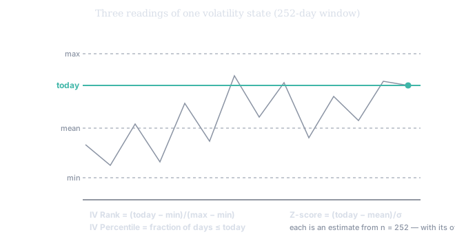
Figure 3. One volatility state, three readings against the 252-day window: IV Rank (position between min and max), IV Percentile (fraction of days at or below today), and the Z-score (distance from the mean in sigmas). They usually agree, but they answer different questions — and every one is an estimate carrying the sampling error of a single year.