Smoothing, Filtering & Trend Extraction
Objectives
- Frame trend extraction as estimating the trend component of price = trend + noise, and see any moving average as a linear filter (a weighted mean whose weights sum to one).
- State the lag-versus-noise (bias-variance) tradeoff that governs every smoother, and explain why it cannot be escaped.
- Explain, statistically, why naive price moving-average crossovers are weak — structural lag, whipsaw, and overfit window lengths (data-snooping).
- Describe EWMA / RiskMetrics variance as exponential smoothing of squared returns and a special integrated GARCH — the genuine quantitative use of smoothing.
- Recognize bias-detrended and adaptive (Kalman / state-space) smoothers as what serious volatility and regime estimation actually relies on.
A single price tells you where the asset is; it does not tell you where it is going, and worse, today's price is contaminated. Buried inside it is a little genuine drift — the trend you care about — and a much larger pile of noise: the spread, the last nervous order, a headline forgotten by Thursday. This chapter is about separating those two. But we are going to treat it as what it actually is — a problem of statistical signal extraction — rather than as a tour of retail moving-average tricks, because almost nothing in serious quantitative work, and very little in Saqrid, rests on a plain moving average of price.
Trend extraction is an estimation problem
The classical way to state the problem (from time-series theory) is to model the observed series as a sum of pieces:
where is a slowly-varying trend and is zero-mean noise. Your goal is to estimate the unobservable from the contaminated . That is all "smoothing" is: an estimator of the trend component. And the oldest such estimator is the average — if one number is noisy, average several and the noise tends to cancel while the trend survives. A moving average is that idea slid along time. But framing it as an estimator immediately tells you its assumptions and its failure modes, which the retail framing hides.
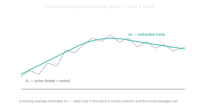
Figure 1. Smoothing is signal extraction. The jagged gray line is the price ; the smooth teal line is the extracted trend . A moving average recovers only under two assumptions: that the trend is roughly linear across the window, and that the noise averages to about zero over it. When either fails — a sharp turn, or autocorrelated noise — the estimate is biased, and no amount of averaging fixes it.
Every moving average is the same object: a linear filter
The retail world catalogues moving averages — simple (SMA), weighted (WMA), exponential (EMA), triangular (TMA) — as if they were different species. Statistically they are one object with different settings. Each is a weighted mean of recent prices whose weights sum to one; equivalently, each is a linear filter, a fixed weight profile dragged across the series:
The SMA makes all weights equal; the WMA tilts them linearly toward the present; the EMA lets them decay geometrically forever, computed by the recursion — itself the textbook definition of exponential smoothing. The constant is just the choice that matches an EMA's center-of-mass (its average lag) to an -day SMA's, so the two are comparable. The TMA averages an average, pushing the weights into a triangle. That is the entire taxonomy, and it is a footnote: choosing a moving average is choosing the shape of one weight profile. Once you see filters as designable, you realize the windowed averages are crude — signal-processing has long built filters with engineered weights (the Spencer 15-point filter, for instance) that smooth far more cleanly than any plain window. The window is the beginning of the subject, not the end.
The one tradeoff that governs every smoother
Every filter faces the same unavoidable bargain, and it is the bias-variance tradeoff from your estimation chapter wearing time-series clothes. A short window averages few points: it has low bias (it tracks the current trend) but high variance (it stays noisy and turns on twitches). A long window averages many: low variance (beautifully smooth) but high bias, here taking the specific form of lag — it reports the trend as it was, not as it is.
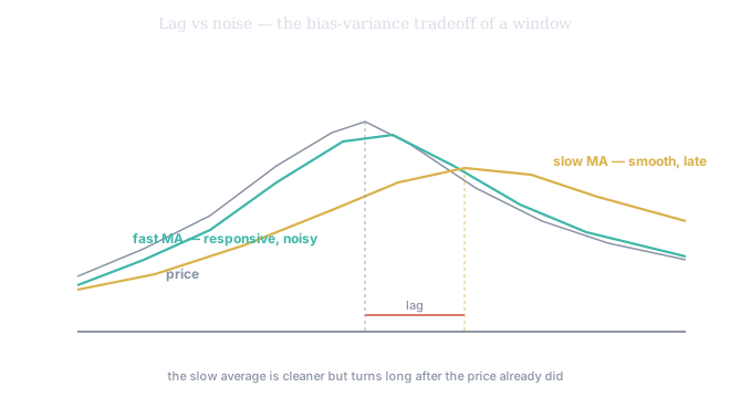
Figure 2. The same price, two windows. The fast filter (teal) turns almost with the price but jitters; the slow filter (gold) is clean but rounds the corner long after the price already turned. That gap is lag, and it is not a flaw to be tuned away — it is structural. A causal filter sees only the past, so any smoothing it buys is paid for in delay. You can move the tradeoff; you cannot escape it.
Why a moving average is not a strategy
Here is the part the indicator culture skips, and the reason Saqrid does not hang its hat on price moving averages. Treated as a trading signal — "buy when the fast MA crosses above the slow" — a moving-average crossover is statistically weak, for three compounding reasons.
First, the lag is structural (Figure 2): a crossover is a comparison of two already-delayed estimates, so it confirms a turn well after it happened. Second, it whipsaws: in a choppy, trendless stretch — which is most of the time — the two lines cross back and forth on noise, generating a stream of false signals, each one a small loss. Third, and most insidious, the window lengths are almost always overfit. Searching history for the (fast, slow) pair that would have made the prettiest backtest is exactly the data-snooping trap from Tier 100 ch6: with two free parameters and thousands of price series, some pair always looks brilliant in-sample and means nothing out-of-sample. A moving average is a legitimate estimate of the trend; it is a poor edge, and reading it as a buy/sell trigger confuses the two. This is precisely why "very few, if any" serious tools rely on plain price MAs — and why we now turn to where smoothing genuinely pays.
Where smoothing actually earns its keep
The quantitative value of these ideas is real — it is just not on the price line. It is on variance, on bias removal, and on adaptation.
Smooth the variance, not the price: EWMA and RiskMetrics
The single most important application of exponential smoothing in finance is not to price at all — it is to volatility. Squared returns are a noisy, unbiased proxy for the instantaneous variance, far too jumpy to use raw. Exponentially smooth them and you get a responsive, stable volatility estimate — the EWMA / RiskMetrics estimator:
It is the EMA recursion applied to instead of . A volatility shock enters immediately (good — you want risk to update fast) yet decays smoothly afterward, with tuning the memory. And it is not an ad-hoc gadget: it is exactly a special "integrated" GARCH model — the persistence pinned to one — which is your direct bridge to the GARCH chapter in Tier 200. This is the smoothing that matters, and it lives under volatility estimation, value-at-risk, and the vol-regime tools you already met.
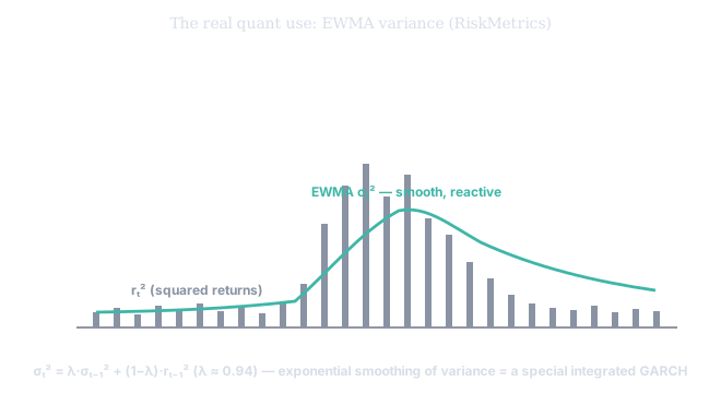
Figure 3. The genuine use. Gray bars are spiky squared returns with a volatility cluster in the middle; the teal line is the EWMA variance riding over them — reacting fast to the burst, decaying gracefully after. The same exponential weighting that makes a mediocre price filter makes an excellent variance filter, because variance genuinely clusters and persists (Tier 100 ch2) in a way price level does not.
Strip the bias: detrended smoothing
Recall from the volatility chapter that a plain close-to-close estimate is biased upward by a trend — a drifting mean masquerades as extra dispersion, and a naive moving average inherits exactly this contamination. The fix is to detrend before you smooth, which is what SV's BHV(P&R) does with its Bayesian bias-detrended core (the nBD moving average): it removes the trend leakage so the smoothed series measures genuine volatility regime rather than the trend faking it. A smoother is only as honest as the bias it removes first.
Let the filter adapt: Kalman and state-space
The deepest limitation of every moving average is that its weights are fixed — it smooths a calm market and a violent one with the same hand. The modern answer is an adaptive filter that adjusts how much it smooths to how noisy the data currently is. The Kalman filter and the broader state-space framework do exactly this: they model the unobserved trend as a hidden state and compute the optimal estimate at each step, leaning on new data when it is informative and ignoring it when it is noise. The Hodrick-Prescott filter and LOESS are cousins. These — not SMA crossovers — are the trend-extraction tools of quantitative finance, and you will build the state-space machinery properly in Tier 200 and beyond. For now, the lesson is the direction of travel: from a fixed window, to a designed filter, to a filter that thinks.
Here is where the smoothing lives in Saqrid. The four price moving averages exist in SV as basic overlays, but the platform's statistical weight is on smoothing volatility and regime series, not price: HV(P&R) smooths its volatility series with an EMA and wraps it in ±1 SE bands (separating a real regime shift from a one-day twitch); BHV(P&R) goes further with bias-detrended smoothing; and the volatility engine is closer in spirit to EWMA/GARCH than to a price average. If you ever find yourself trading a raw price MA crossover, the platform is quietly pointing you somewhere better: smooth the risk, detrend the bias, and let the filter adapt.