Portfolio Mathematics: Two-Asset to N-Asset Risk
Objectives
- Compute a portfolio's expected return (wᵀμ) and the two-asset variance with its covariance cross-term, and explain why risk is not the weighted average of its parts.
- Generalize portfolio variance to N assets as the quadratic form wᵀΣw using the covariance matrix.
- State the Markowitz problem and read the efficient frontier and the minimum-variance portfolio.
- Decompose total risk into diversifiable (idiosyncratic) and non-diversifiable (systematic) parts, and explain the systematic floor.
- Name the honest weaknesses of mean-variance optimization — estimation error in μ, correlations rising to one in crises, and variance understating tail risk.
Here is the most important free lunch in all of finance, and it is going to look, at first, like cheating. Take two assets that each swing by the same amount — the same volatility, the same risk. Put half your money in each. You might expect the combined risk to be that same amount; you have not made either asset calmer. But if the two do not move in perfect lockstep, the risk of the blend is lower than the risk of either piece. You reduced risk without reducing expected return. That is diversification, the only thing in this field that genuinely gives you something for nothing — and this capstone of 102 is about the exact mathematics that makes it real.
Expected return: the boring part
Hold a fraction of your money in asset 1 and in asset 2, with . The expected return of the portfolio is just the weighted average of the expected returns — a direct consequence of the linearity of expectation from ch1:
Sixty percent in something expecting 8% and 40% in something expecting 4% gives . Returns blend by straight weighting — no covariance, nothing clever. Expected return is the boring part.
Risk: the covariance cross-term
Risk is where it gets interesting, because variance does not blend by straight weighting. The two-asset portfolio variance is
Read that last term slowly, because it is the entire story. It carries the covariance between the assets () — whether they move together. Positive covariance adds to your risk; negative covariance subtracts from it. If the assets move in perfect opposition, that subtraction can crush the portfolio variance — in the extreme, all the way to zero. Your risk is not the average of the two risks; it is that average, adjusted by how the pieces co-move. You cannot choose the means by cleverness, but you absolutely get to choose how the pieces interact.
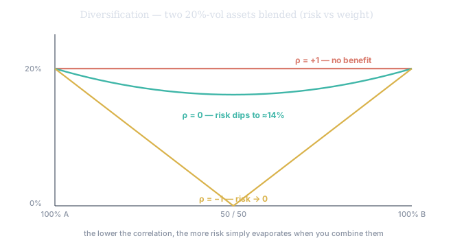
Figure 1. Two assets, each 20% volatility, blended by weight. At ρ = +1 the line is flat at 20% — the assets are copies, the cross-term is fully additive, no benefit. At ρ = 0 the risk dips to ≈14% at the 50/50 blend. At ρ = −1 it collapses to zero at the right weights. The lower the correlation, the more risk simply evaporates. This curve is diversification, drawn.
Correlation scales the benefit
Covariance has awkward units (returns-squared), so we normalize it to correlation, . At the assets are perfect copies and the portfolio risk is the weighted average — the free lunch vanishes. At they're unrelated. At they perfectly offset and a careful blend is risk-free. Every real pair lives in between, and the closer to you get, the more risk disappears when you combine them.
Scaling up: the covariance matrix
Two assets was a warm-up; a real portfolio holds many, and the structure stays identical while the bookkeeping explodes. Expected return is still . The variance is still a sum of variance terms plus a covariance term for every pair — but ten assets have 45 pairs and a hundred have nearly 5,000. You collect every variance and pairwise covariance into one object, the covariance matrix (variances on the diagonal, covariances off it), and the entire portfolio variance compresses to a single quadratic form:
One line of linear algebra holds all 5,000 interactions at once. And it reframes the institute's throughline: a single asset's volatility is not evidence of your portfolio's risk. The risk lives in — in how the holdings move relative to each other. An asset that looks dangerous alone can lower your total risk if it leans against the rest. Risk is a property of the whole, never of the parts in isolation.
The efficient frontier
With and in hand, Markowitz mean-variance optimization asks one precise question: for each target expected return, which weights give the smallest possible variance?
This is a convex quadratic program (you'll meet the optimization machinery formally in Tier 300), and sweeping across all levels traces the efficient frontier.
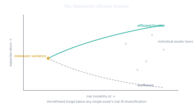
Figure 2. Every point on the teal frontier is a portfolio you cannot improve — no more return without more risk, no less risk without giving up return. The gold vertex is the minimum-variance portfolio. Individual assets sit inside and to the right (more risk for their return). The frontier bulges left, into lower risk than any single asset offers — and that leftward bulge is the covariance cross-terms doing their subtraction, drawn as a picture.
The mean-variance optimizer in SVQ works on a handful of assets at a time. Behind the screen it estimates each asset's expected return and the covariance matrix from this chapter, then sweeps the min-variance question across return levels to plot the efficient frontier. The leftward bulge below any single asset's risk is the diversification. As the target return moves along the curve, the weights rebalance — that is the quadratic program re-solving live.
What diversification can — and cannot — do
Diversification is powerful but not unlimited, and the limit is one of the most important facts in finance. Take equally-weighted assets, each with average variance and average pairwise covariance . The portfolio variance works out to
Read the two pieces. The first, , is idiosyncratic risk — the asset-specific noise — and it vanishes as you add names (a stock's own surprises wash out in a big enough basket). The second, , is systematic risk — the shared, market-wide co-movement — and it does not go away no matter how many assets you hold. Diversification eliminates the diversifiable and leaves a floor.
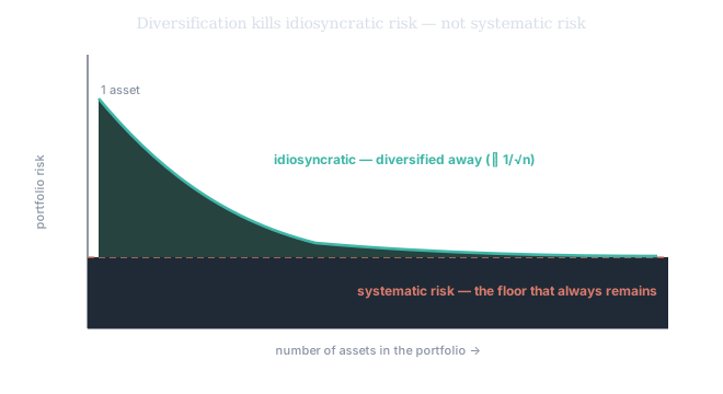
Figure 3. Portfolio risk versus the number of holdings. It falls steeply at first — idiosyncratic risk diversifying away roughly like — then flattens onto the systematic floor it can never breach. The shrinking teal gap is the risk you can remove for free; the red floor is the market risk you are paid to bear. This single picture is the seed of the CAPM and factor models you'll build in the advanced tiers.
The honest caveats
Markowitz is the right place to start portfolio construction and the wrong place to stop — for three reasons you are now equipped to see.
First, the inputs are estimates, and one of them is barely knowable. Expected returns carry enormous standard errors (ch5 of Tier 100: the mean is the hardest moment to pin down). The optimizer, handed noisy 's, tilts aggressively toward whatever asset looks best — which is often just estimation noise. Critics rightly call naive mean-variance an "error-maximizing" machine: tiny input changes swing the weights wildly. The fixes — shrinkage, resampling, constraints — all amount to distrusting your own estimates.
Second, the covariance matrix is not stationary, and it betrays you in crises. Correlations that look comfortably low in calm markets rush toward in a crash (ch3 of Tier 100), so the diversification you counted on evaporates exactly when you need it. That tail-correlation behavior is why the advanced tiers reach past correlation to copulas and contagion models.
Third, variance is not the whole of risk. Mean-variance treats a big gain and a big loss symmetrically, but returns are fat-tailed and negatively skewed (ch2 of Tier 100), so variance understates the danger that actually ruins portfolios. The repair is to optimize a genuine tail measure — Conditional Value-at-Risk — which you'll build in Tier 400.
Closing Tier 100's probability course
This completes 102, and with it the probabilistic foundation. You started with a single uncertain number — the random variable (ch1) — gave it the normal-lognormal return model (ch2), learned to update it by conditioning (ch3), to measure its volatility honestly (ch4), to extract its trend without being fooled (ch5), and now to assemble many of them into a portfolio whose risk lives not in any asset but in the matrix of how they all move together. The single thread: risk is a property of the whole distribution, and of the whole portfolio — never of a number in isolation. Tier 200 makes the estimation behind every one of these objects rigorous — inference, regression, and the GARCH volatility models that the EWMA of last chapter only previewed.