Conditional Probability, Bayes & Expectation
Objectives
- Compute conditional probabilities and conditional expectations, and relate them through joint, marginal, and conditional distributions.
- State Bayes' rule and separate the likelihood from the prior (base rate).
- Explain why E[X|Y] is a random variable — the best forecast of X given Y, and the regression function.
- Apply the law of iterated expectations and the law of total variance, and identify explained vs unexplained variance (the seed of R²).
- Read the SVQ probability cone as a stack of conditional distributions and explain why conditioning on a useful signal narrows it.
Everything you believe about a market is conditional on something. When you say an asset has a 60% chance of finishing the week higher, that number is never floating free — it sits on a pile of facts you're holding fixed: today's price, this week's volatility, that earnings already came out. Change any one and the 60% changes with it. This is the most important idea in the probability of returns, and it has a precise name: conditional probability — the probability of one thing given that you already know another. This chapter builds it into the full predictive engine — conditional expectation — that 102's regression and forecasting all rest on.
Conditioning is throwing away worlds
Build the intuition before the symbols. Imagine all the ways next week could unfold as a giant bag of possible worlds. Unconditionally, you reach into the whole bag. The moment you learn something true — say, the price is already up 2% by Tuesday — you throw away every world inconsistent with that fact and reach only into the survivors. The probability of a Friday close above some level, given the Tuesday move, is the fraction of those surviving worlds in which it happens. Conditioning is throwing away worlds. That is all it is. The formula says exactly that:
You take the slice where both are true and re-weight by how big the -slice was, because is your new universe — dividing by makes the survivors add back to one.
Joint, marginal, conditional
To handle two uncertain quantities at once — say a Tuesday move and a Friday return — you need their joint distribution , the probability of each pair. From it, two things drop out. The marginal is what you get by ignoring one variable (sum or integrate it away): — the distribution of alone. The conditional is what you get by fixing one variable: — the distribution of once is known. Marginal is forgetting; conditional is learning. The whole chapter is the difference between those two operations.
Bayes' rule
From the one definition comes the most useful updating tool, Bayes' rule. It answers the question markets actually pose, which runs backwards from how data arrives: you observe an effect — a sharp move, a volume spike — and want the probability of a cause (the trend has genuinely turned). What you can estimate is the other direction: if the trend had turned, how likely was this move? Bayes flips one into the other —
The piece beginners forget is the prior, the base rate. A signal that's right 80% of the time when a real breakout is underway sounds impressive — until you remember breakouts are rare, maybe one day in twenty. Run it through Bayes and the chance this firing is real can still be modest, because the tiny prior drags it down (you proved this numerically in Tier 100 ch4). Before acting on a number, always ask what it was conditional on, and what the base rate was underneath.
Conditional expectation: the best forecast
Alongside conditional probability sits the idea this course is really after: conditional expectation. Where conditional probability gives the chance of an event among the surviving worlds, conditional expectation gives the average value of some quantity across them:
Fix , restrict to the worlds where it holds, average over what remains. This is the single best forecast of once is known — "best" in the precise sense that it minimizes average squared error. No other function of predicts with smaller expected squared miss. That is a strong claim, and it is why conditional expectation is the theoretical target of all of forecasting.
Now the subtle point that elevates this above ch1's expectation. is a number once you plug in a specific — but before you observe , it is a function of , and therefore itself a random variable, written . Its value is whatever the conditional mean happens to be once lands. Read as a function of the conditioning variable, is exactly the regression function — the curve that gives the best -prediction at each — which is why estimating it from data is the entire subject of Tier 200's regression.
![*Figure 1.* Conditioning, drawn. The cloud is the joint distribution of two variables. Fix $X$ at $x_0$ and you keep only the highlighted vertical slice — that's the **conditional distribution** of $Y$ given $X=x_0$. Its average is $\mathbb{E}[Y\mid X=x_0]$ (the gold dot), and as $x_0$ slides across, those conditional means trace the teal **regression function** $\mathbb{E}[Y\mid X]$. This one picture *is* conditional expectation, and it is the object Tier 200 will learn to fit.](/figures/conditional-slice.svg)
Figure 1. Conditioning, drawn. The cloud is the joint distribution of two variables. Fix at and you keep only the highlighted vertical slice — that's the conditional distribution of given . Its average is (the gold dot), and as slides across, those conditional means trace the teal regression function . This one picture is conditional expectation, and it is the object Tier 200 will learn to fit.
The tower rule: iterated expectations
Conditional and unconditional expectations are tied by one elegant identity, the law of iterated expectations (the "tower rule"):
In words: the average of the conditional averages is the grand average. Average the Friday return within each possible Tuesday move, then average those across all Tuesday moves weighted by how often each occurs, and you recover the plain expected Friday return. It is both a sanity check (conditioning can't manufacture or destroy the overall mean) and a practical computing trick — hard expectations often crack open when you compute them in two stages, inner then outer.
How much did conditioning actually help? Total variance
Iterated expectations says conditioning leaves the mean alone. The deeper question is what conditioning does to uncertainty — and the answer is the law of total variance, the most important equation in this chapter:
Total uncertainty in splits cleanly into two pieces. The unexplained part is the average leftover scatter within each -slice — the noise conditioning can't remove. The explained part is how much the conditional mean itself moves as varies — the uncertainty conditioning resolves. A predictor that genuinely knows something makes swing widely (large explained) and leaves little residual scatter (small unexplained). The fraction is exactly the R² you'll meet in regression — the share of variance a signal accounts for.
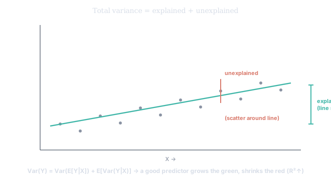
Figure 2. The split, made visible. Explained variance is the rise of the regression line across — the conditional means genuinely differ. Unexplained variance is the scatter of points around that line within any slice — what the predictor still can't tell you. A better predictor grows the green and shrinks the red. This is the precise sense in which "information reduces uncertainty," and it is the entire economic value of any signal.
The limiting case names itself: if and are independent, then — a flat line, no rise — so the explained variance is zero. Conditioning on an independent variable tells you nothing, and the cone doesn't budge. Independence is the formal statement of "this signal is useless."
The cone is conditional belief, drawn
This is the exact machinery under one of SVQ's most-used outputs.
The SVQ probability cone fans from today's price into the future as shaded bands that widen with the horizon. It is a stack of conditional distributions: at each forward date, SVQ holds today's price and the current volatility fixed and asks, given those, what is the distribution of where the asset could be? The centerline is the conditional expectation — the average landing spot given those conditions. The inner band holds the central ~68% of that conditional distribution, the outer ~95%. The cone widens not because conditioning admits more worlds (it never does) but because the conditional variance of the terminal price grows with the horizon — the σ√t rule from ch2, curving the edges outward. The cone is not a prediction of one path; it is the shape of your conditional belief. Where it pays off: when price pokes outside the outer band, that is the likelihood term screaming — under the model, an excursion this large was supposed to be rare. Bayes then says update: either a genuine regime shift is underway, or volatility jumped and the cone was too narrow. A move beyond the band demands a new posterior; a move comfortably inside is noise, fully consistent with the prior, and should move your beliefs hardly at all.
And here is the deeper lever, straight from the total-variance law. The standard cone conditions only on price and volatility. Feed it a genuinely informative signal — condition on something that moves — and the band should tighten, because you've converted unexplained variance into explained.
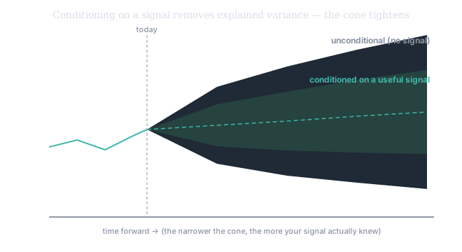
Figure 3. The wide cone is unconditional (no signal). The narrow cone is what's left after conditioning on a useful predictor: the explained variance has been removed, so less uncertainty remains. The amount a cone tightens when you add a signal is a direct, visual measure of how much that signal actually knew — which, formally, is its share of the total variance.