The Normal & Lognormal Return Model
Objectives
- State the normal-log-return / lognormal-price model, write the normal density, and explain why prices are lognormal and floored at zero.
- Use μ, σ and normal quantiles (the 68-95-99.7 rule, ±1.96σ) to build forward price bands, and scale them with the √t rule.
- Describe geometric Brownian motion and separate its drift (μ) from its diffusion (σ).
- Explain the volatility drag: why the forward (mean) price sits above the median, via the −σ²/2 adjustment.
- Read a SVQ probability tunnel as a distributional statement, and name the assumptions (fat tails, skew) that make it understate risk.
In the last chapter you built the random variable and met the distribution catalogue. Now we commit to the two distributions that carry almost all of practical finance — the normal for returns and the lognormal for prices — and assemble them into the single model that SVQ's probability tunnel and SV's Normal Cone actually draw. A single return tells you what happened once; a model of returns tells you what tends to happen, and that is the thing you can bet on.
The normal distribution
Pile an asset's daily log-returns into a histogram and you get a familiar shape: most days cluster near zero, big moves are rarer the bigger they get, and they fall off roughly symmetrically on each side. That bell is so common, and so convenient, that the foundation of quantitative finance is built on approximating it with one curve — the normal distribution, written , with density
It is fully described by just two numbers: the center (the return you expect on average) and the spread (the typical size of the surprise — which in finance is volatility). Two numbers, and you have committed to a complete description of the randomness. That economy is the whole appeal — but it is not the only reason the normal is the default. Three reasons stack up: the Central Limit Theorem (Tier 100 ch5) says sums and averages of many small shocks tend toward the normal regardless of the pieces; the two-parameter economy means you only ever estimate and ; and the analytic tractability of the normal gives closed-form answers (it is what makes Black–Scholes solvable). Convenience, justification, and tractability all point the same way.
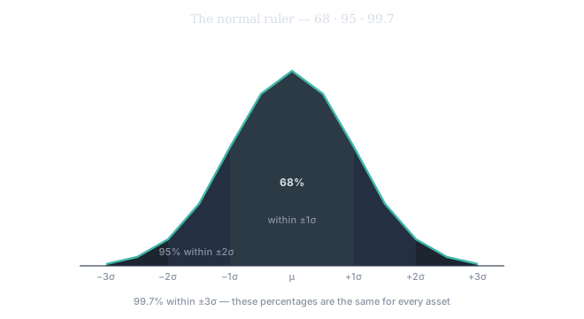
Figure 1. The defining property: probability sits around the mean in fixed multiples of σ. About 68% of draws land within ±1σ, 95% within ±2σ (1.96σ to be exact), 99.7% within ±3σ. These percentages don't depend on the asset — they are a property of the curve. So once you've estimated μ and σ, you have the probability of every outcome.
The standard normal and quantiles
Strip a normal of its particular μ and σ by standardizing — from last chapter — and you get the standard normal , denoted , with density and CDF . Every normal question reduces to a question about this one universal curve. That is the engine behind a quantile — the value below which a stated fraction of the distribution falls. For the normal these are tabulated multiples of σ: the 2.5th and 97.5th percentiles sit at from the mean and bracket the middle 95% of outcomes. Pick a confidence level, look up the matching σ-multiple, and you can draw a band the future return should stay inside with exactly that probability — if the model holds.
From normal returns to lognormal prices
Now watch what the assumption does to prices. You modeled the log-return as normal — but the log-return is the natural log of tomorrow's price over today's. If the log of the price ratio is normal, the price ratio itself is the exponential of a normal, and a quantity whose logarithm is normal is lognormal. From ch1: a function of a random variable is a random variable, and here the function is .
So one assumption gives two views at once. Log-returns are normal — symmetric, and free to be negative. Prices are lognormal — skewed right, and never below zero. That second fact isn't a rule you memorize separately; it falls straight out of the model, because you cannot take the log of a negative number. An asset can lose at most all its value, but a price of −10 is meaningless, and the lognormal respects that floor for free.
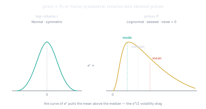
Figure 2. The exponential map. A symmetric normal of log-returns (left) becomes, through , a right-skewed lognormal of prices (right) with a hard floor at zero. Notice the three centers no longer coincide: mode < median < mean. The curve of stretches the up-moves more than the down-moves, dragging the mean to the right of the typical outcome — a gap we are about to name and measure.
Geometric Brownian motion: the model in motion
So far the model is a snapshot. The dynamic version — the one the cone is built on — is geometric Brownian motion (GBM), the standard continuous-time model of a price:
Read it as two forces. The drift term is the deterministic pull — the average growth rate compounding the price upward. The diffusion term is the random buffeting — scaling a stream of independent normal shocks (). Drift is where the price is headed; diffusion is how much it wanders on the way. The defining feature of GBM is that these act proportionally to the price (a stock at 200 moves twice as many dollars as one at 100), which is exactly why returns, not price changes, are the natural unit — and why the solution makes log-returns normal: over a horizon , is normally distributed. That is the model's beating heart.
The volatility drag: why the forward sits above the median
GBM hides a subtle and important fact, and it is where this chapter earns its keep. Solving the equation, the log-return over horizon is normal not with mean but with mean :
That is the volatility drag, and it produces the mode-median-mean ordering you saw in Figure 2. The median price — the typical, middle outcome — grows at the reduced rate: . The mean price — the probability-weighted average, the forward — grows at the full rate: . The gap between them is exactly the drag, .
Why does volatility subtract from the typical growth? Because compounding is asymmetric: a −50% move needs a +100% move to recover (ch1's first lesson), so the up-and-down jostling of volatility erodes the compounded path even when the average arithmetic return is positive. The mean is pulled up by a handful of enormous winning paths (the fat right edge of the lognormal); the path you'll actually tend to experience is the median, growing slower by . This is the rigorous version of the geometric-vs-arithmetic gap from ch1, and the formal payoff of the Jensen's-inequality preview: because is curved, . Higher volatility, bigger drag — a fact that quietly governs leveraged products, rebalancing, and why a volatile asset with a positive average return can still bleed.
Scaling to the horizon: the √t cone
One day or many, the same engine scales. Because log-returns add across time, their variances add, so the standard deviation of an -day return grows as — the square-root-of-time rule. A band ten days out is not ten times a one-day band; it is about times as wide. Uncertainty grows, but sub-linearly, and the set of plausible prices fans out like the square root of the horizon.
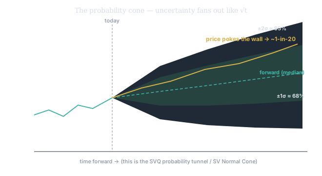
Figure 3. The model rendered forward. From today, the forward (median) line drifts up, and the ±1σ (≈68%) and ±2σ (≈95%) bands flare outward as √t. A future price that pokes the outer wall is — under the model — a roughly 1-in-20 event. This cone is the SVQ probability tunnel and SV's Normal Cone: the entire normal-lognormal model, drawn.
This is exactly what the SVQ probability tunnel draws. SVQ takes the asset's log-returns, estimates the volatility σ, and projects a forward price — the model's center at each future date. Around it, it lays normal-quantile bands: the inner band ≈ ±1σ (about 68% of modeled outcomes), the outer ≈ ±1.96σ (the 95% band). Because the width scales as √t, the tunnel flares as you look further forward — the √t rule on screen. And because the lognormal is right-skewed, the true mean (forward) price sits slightly above the median line by the σ²/2 drag you just derived — symmetric in log space, skewed in price space. So when price pokes outside the outer wall, the model is telling you that, under the normal assumption, this was a roughly one-in-twenty event: your first piece of genuine, quantified evidence that something unusual is happening — a probability, not a hunch.
The honesty clause
This model is an approximation, and you should know exactly where it lies to you. Real return distributions have fat tails — extreme moves happen more often than the normal predicts (Tier 100 ch2) — and they often have skew, with crashes outrunning rallies. So the true odds of touching the outer tunnel wall are usually a little higher than the clean 5% suggests. The normal-lognormal model is the right place to start reasoning, the default lens SVQ hands you, and a disciplined baseline against which to judge a number. Everything in the advanced tiers is a correction to it: the Student-t and GARCH repair the tails and the clustering, the volatility surface repairs the skew. A move that breaches the band is evidence precisely because the model says it should be rare — and knowing the model's blind spots is what keeps you from trusting that evidence too much.