Random Variables & Probability Foundations
Objectives
- Define a random variable formally as a map from outcomes to numbers, and distinguish discrete (PMF) from continuous (PDF) variables.
- Read probability as area under a density, know that P(X=x)=0 for a continuous variable, and read the CDF as the object that contains everything.
- Compute expectation and variance as operators (sum and integral forms) and apply their algebra — linearity and the a² scaling law.
- Name the distribution catalogue used to model returns, and explain why normal log-returns make prices lognormal.
- Standardize any value into a z-score and use it as the universal ruler for 'is this move large?'
You already know that finance runs on returns, not prices. Now we confront the harder truth about a return: before it happens, you do not know what it will be. Tomorrow's return is not a number you can look up — it is a number that could land anywhere across a range of possibilities, each with its own chance. The whole of quantitative finance is the discipline of reasoning carefully about that not-yet-known number, and Tier 100's first course gave you the statistics to read such numbers after the fact. This course, SVI 102, gives you the probability that generates them — the formal models from which returns are drawn. It begins with the object that makes uncertainty precise: the random variable.
What a random variable actually is
Informally, a random variable is a quantity whose value is set by the outcome of something uncertain — tomorrow's return, a die roll, the number of up-days next week. Formally, and this is worth stating once properly, a random variable is a map from outcomes to numbers: write it , where is the set of all possible outcomes and assigns a real number to each. Flip a coin ten times; let be the number of heads; then the outcome HHTHHTHHTT is mapped to the number 6. The sample space is always there, lurking behind the variable, even once we stop mentioning it and work with directly.
What lifts a random variable above a vague feeling of uncertainty is that it carries a distribution: a complete accounting of which values are possible and how much probability sits on each. The values are one thing; the probabilities are a separate thing. Keeping those apart is the first habit of a quantitative thinker — a value tells you what could happen, a probability tells you how seriously to take it. And random variables come in two species, depending on what the set of possible values looks like.
Discrete variables: probability sits on points
A discrete random variable takes a countable set of separate values — 0, 1, 2 heads; an up day or a down day. Its distribution is given by a probability mass function (PMF), , the probability sitting on each value.
Make it concrete with a deliberately simple asset. Suppose tomorrow's return can take only three values: it rises 2% with probability 0.5, stays flat at 0% with probability 0.3, and falls 3% with probability 0.2. The probabilities sum to one — — because something must happen. That is not optional; it is the defining rule of any distribution, discrete or continuous. Every distribution you will ever meet obeys it.
Continuous variables: probability is area
But a real return is not three values — it is any value on a continuum. For a continuous random variable the probability of landing on any exact value is zero ( — there are infinitely many possibilities, so no single one carries weight), and we describe it instead with a probability density function (PDF), . The density is not itself a probability; probability is the area under it. The chance the return lands between and is the integral
and the total area is one, — the continuous echo of "the probabilities sum to one."
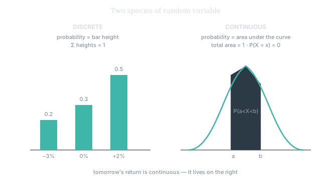
Figure 1. The two species. On the left, a discrete variable: probability is the height of a bar on each value, and the heights sum to 1. On the right, a continuous variable: probability is the area under a smooth density between two points, and the total area is 1. Tomorrow's return lives on the right — which is why, from here on, the smooth density is our basic picture of "a return."
This is the conceptual jump that all of 102 rests on. In Tier 100's foundations you looked at samples — histograms of returns that already happened. Here we look at the density the returns are drawn from: the idealized, infinitely-fine shape behind the histogram. The histogram was the data; the density is the model.
The CDF: the one object that contains everything
Discrete and continuous variables seem to need different descriptions — a PMF for one, a PDF for the other. But there is a single object that handles both and, remarkably, contains all the information about a random variable: the cumulative distribution function (CDF),
It answers one question for every level : how much probability lies at or below it? For a continuous variable, is exactly the area under the density up to — so the CDF and the PDF are two views of the same thing, the CDF being the running total of the density. Every CDF shares three properties: it never decreases, it rises from 0 (far left) to 1 (far right), and it is right-continuous. Hand someone the CDF and they can recover any probability you like — which is why it, not the density, is the theoretically fundamental object.
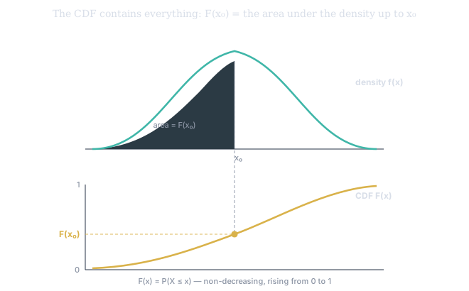
Figure 2. Top: a density, with the area up to a point shaded. Bottom: the CDF, an S-shaped climb from 0 to 1. The height of the CDF at equals the shaded area above it — that's the definition made visual. Every quantile you'll ever read (the median, a Value-at-Risk level, an IV percentile) is just this curve, read backwards: pick a probability on the vertical axis, slide across, read off the value.
Expectation: the operator for the center
With the variable defined, we ask the two questions that organize everything: where is it centered, and how spread out is it? The center is the expectation — the probability-weighted average of the outcomes. For our discrete asset, multiply each value by its probability and add: . For a continuous variable the sum becomes an integral, — same idea, weighting each value by its density.
Think of as an operator — a machine that takes a random variable and returns its center — because its single most useful property is how it behaves under arithmetic. Expectation is linear:
and the second part holds whether or not and are related. This is the quiet workhorse behind portfolio math (the expected return of a portfolio is just the weighted average of its holdings' expected returns) and we will lean on it constantly.
One trap, worth a permanent warning. The expectation is not the most likely outcome, and need not even be a value the variable can take. Our asset's single most likely return is +2%, but its expectation is +0.4% — dragged down by the real chance of a loss. The expectation is a weighted center of gravity, not a popular vote. Confusing the average with the typical is one of the most expensive mistakes in this field, and you have now been warned about it on day one.
Variance and standard deviation: the operator for spread
The spread is the variance: the expected squared distance from the mean,
We square the deviations because raw distances above and below the mean would cancel, and because squaring punishes the large misses that hurt most. Variance lives in squared units (squared percent — meaningless to intuition), so we take its square root and get the standard deviation , back in the variable's own units. As an operator, variance has its own algebra — and note how it differs from expectation's:
Adding a constant shifts the center but changes spread not at all; scaling by multiplies variance by and standard deviation by . Double a position and you double its volatility but quadruple its variance — the asymmetry that makes leverage treacherous.
Standard deviation is the single most useful number in this course, because it is the natural ruler for the question the whole institute is built around: is this move large? A 1% move means nothing in the abstract. It is small if and enormous if . Standard deviation is how you convert a raw number into evidence.
A catalogue of distributions
You will not invent a new distribution for every problem. A small, recurring cast does most of the work, and naming them is half of modeling. Each is a specific shape with a couple of tuning parameters.
** (the bell — our default for log-returns), and the **[lognormal](https://en.wikipedia.org/wiki/Log-normal_distribution)** (right-skewed, never negative — our default for prices). Add the **Student-t** (the Normal's fat-tailed cousin from Tier 100) and you have nearly the whole toolkit of 102.](/figures/distribution-zoo.svg)
Figure 3. The working vocabulary. Discrete: the Bernoulli (a single up-or-down event), the Binomial (the number of up-days in ), the Poisson (counts of rare events — jumps, shocks). Continuous: the Uniform (every value equally likely — pure ignorance), the Normal (the bell — our default for log-returns), and the lognormal (right-skewed, never negative — our default for prices). Add the Student-t (the Normal's fat-tailed cousin from Tier 100) and you have nearly the whole toolkit of 102.
The next chapter is devoted to the two that matter most for returns — the Normal and the lognormal — but it's worth seeing now why they come as a pair.
Functions of random variables: how prices become lognormal
Here is an idea with enormous reach: a function of a random variable is itself a random variable. If is uncertain, then — square it, exponentiate it, take its log — is a new uncertain quantity with its own distribution, inherited from 's.
This is exactly the bridge between returns and prices. A log-return is , so the price ratio is the exponential of the return: . The exponential is a function, . So if the log-return is Normally distributed, the price — being scaled — is lognormally distributed: skewed right, and never negative, exactly as a price should be. That single move, "prices are the exponential of normal log-returns," is the seed of the Black–Scholes model and of SV's Normal Cone, and you now see precisely where it comes from. (A subtlety for later: because is curved, — the average price is not the price at the average return. That gap, Jensen's inequality, will matter when we price options.)
Standardize: the universal ruler
We close with the operation that turns all of this into a single, portable number. Take any variable, subtract its mean, divide by its standard deviation:
The result — the z-score — has mean 0 and standard deviation 1, and it measures how many standard deviations from the center a value sits, in units that are comparable across any asset, any timeframe, any distribution. A of is a Tuesday; the distribution produces moves like that constantly. A of is the data quietly telling you that, under the asset's own distribution, today was not business as usual. Expectation tells you where the center is; standard deviation tells you what counts as far from it; the z-score fuses them into the first real signal you will ever compute — and it is the seed of every volatility band, IV percentile, and z-score readout in Saqrid.
Any asset's daily log-returns in SV or SVQ are a sample of one underlying random variable. Its mean estimates the expectation; its standard deviation estimates the spread. Today's move, minus the mean, divided by the standard deviation, is a z-score. A reading of is ordinary; a reading of is the platform signaling that today was a genuine outlier under the asset's own distribution. That single ratio is the seed of the z-scores, IV Rank / IV Percentile, and Normal Expected Move bands found across the suite — and the lognormal-price idea above is the foundation under the Normal Cone.