Sampling and Estimation: Why Your Numbers Are Uncertain
Objectives
- Distinguish a population parameter from a sample estimate, and describe the sampling distribution.
- Judge an estimator by bias, variance, and mean-squared error, and explain consistency.
- State the Central Limit Theorem and explain why it lets us put Normal-based error bars on estimates — even for fat-tailed returns.
- Construct and correctly interpret a confidence interval, and state what it does NOT mean.
- Apply the bias–variance tradeoff to the volatility lookback-window choice, and use the bootstrap when formulas fail.
There is a quiet lie built into every number on every trading screen, and once you see it you cannot unsee it. The lie is the appearance of certainty. When the platform tells you an asset's volatility is twenty-two percent, it presents that as a fact, a crisp single value. It is not. It is an estimate, computed from a finite stretch of history, and if you had handed the platform a slightly different stretch it would have told you something slightly different. This chapter is about taking that uncertainty seriously — which, more than any single technique, is what separates a professional from an amateur with a charting app.
Parameter, sample, estimate
The distinction the whole of statistics rests on is this. There is a true, underlying quantity — call it the parameter — that you would know if you had infinite data: the asset's real volatility, its real mean return, its real correlation with something else. You never have infinite data. You have a sample: the particular window of days you happened to look at. From that sample you compute an estimate of the parameter, written with a "hat" — for the parameter . The estimate is what you see. The parameter is what you wanted. They are not the same thing, and the distance between them is where most overconfidence in markets is born.
Because the estimate depends on which sample you drew, it would have come out differently with a different sample. Imagine — as a thought experiment — drawing many independent samples and computing on each. Those estimates would themselves form a distribution: the sampling distribution. This is the single most important idea in the chapter. Your one estimate is a single draw from this distribution; understanding estimation means understanding the shape, center, and spread of the distribution your number came from.
What makes an estimate good: bias, variance, MSE
With the sampling distribution in hand, we can say precisely what "a good estimate" means. Two things can go wrong, and they are independent.
The bias is whether the sampling distribution is centered on the truth: . A biased estimator is systematically too high or too low — it misses in the same direction no matter how much data you feed it. An unbiased one is centered on the target on average. (This is why we divided by in Chapter 3: it removes the bias from the sample variance.)
The variance is how widely the sampling distribution spreads — how much bounces from sample to sample. Low variance means a steady, repeatable number; high variance means a jumpy one you can't trust from one window to the next.
You want both small, and the single number that combines them is the mean-squared error, with a decomposition you should memorize because it governs an enormous amount of practical modeling:
Total error is bias-squared plus variance. An estimator is consistent when both pieces vanish as the sample grows — bias and variance , so the estimate homes in on the truth. Consistency is the formal promise behind "more data helps," and it is the estimation-theory cousin of the Law of Large Numbers from Chapter 4.
The standard error and the √n rule
The square root of that variance — the spread of the sampling distribution — has a name you met in Chapter 3: the standard error (SE). It is not the standard deviation of the data; it is the standard deviation of your estimate. For the sample mean it is , and that in the denominator is the rule with enormous practical consequences: the standard error shrinks with the square root of the sample size.
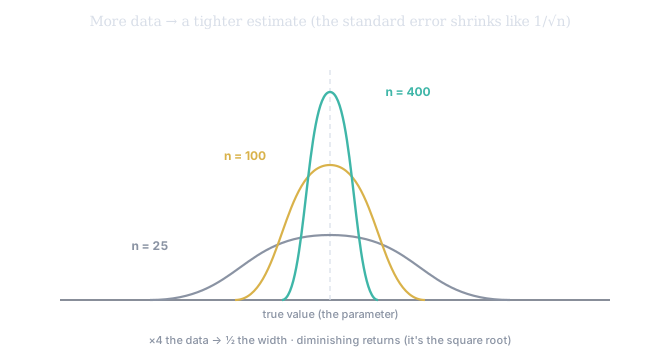
Figure 1. The same estimate computed on bigger and bigger samples. The sampling distribution stays centered on the truth but tightens as grows. Quadruple the data and the spread halves — and because it's a square root, the returns diminish: doubling your window does not double your confidence. This is why a 5-day volatility jumps around while a 60-day one sits still.
The Central Limit Theorem — why any of this works
Here is the deep question we've been dancing around. We keep wanting to draw bell curves around estimates and talk about "95%." But returns themselves are fat-tailed and skewed — Chapter 2 hammered that home. So what gives us the right to use the Normal distribution at all?
The answer is one of the most remarkable results in all of mathematics, the Central Limit Theorem (CLT). It says: if you average independent draws from almost any distribution — with any shape, skewed, fat-tailed, lumpy, it does not matter — the average is approximately Normally distributed for large :
Read that carefully. The individual returns can be as non-Normal as they like; the sample mean (and, it turns out, most well-behaved estimators) is approximately Normal anyway. The CLT is what lets us attach Normal-based error bars to estimates even when the raw data is anything but Normal. It is the bridge from the messy real distribution to the clean machinery of confidence intervals.
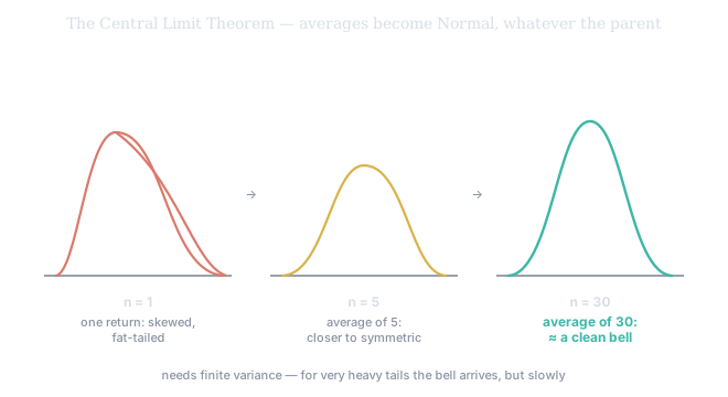
Figure 2. A single return is skewed and fat-tailed (left). But average five of them and the lumps smooth out; average thirty and the distribution of that average is essentially a clean bell (right) — no matter how ugly the parent. That is the CLT, and it is why "the estimate is approximately Normal" is a safe default.
One honest caveat, and it's a deep one. The CLT needs the distribution to have a finite variance. For the moderately fat tails of ordinary returns, that holds — but the fatter the tails, the slower the bell arrives, so on small samples of turbulent data the Normal approximation is rough. And for the truly extreme tails some markets flirt with (the infinite-variance regime from Chapter 2's stable distributions), the CLT can fail outright. This is exactly why tail risk gets its own machinery — extreme-value theory — in Tier 400, rather than trusting the bell in the one place it's weakest.
Confidence intervals, done right
The standard error plus the CLT let us do the honest thing: report an estimate not as a point but as a confidence interval. Because the estimate is approximately Normal, a 95% interval is built by reaching out about two standard errors on each side:
where the is the point on the standard Normal that brackets the middle 95% (two SEs, near enough, for back-of-envelope work). Make it concrete with our volatility. Suppose the estimate is 22% and, given the window length, its standard error works out to about 4 percentage points. Then the 95% interval is , i.e. roughly 14% to 30%. The crisp "volatility is 22%" becomes the truthful "volatility is somewhere around 22%, plausibly between 14 and 30" — and that width is the actual information content.
Now the misreading, because nearly everyone makes it and you must not. It is tempting to say "there is a 95% chance the true value lies inside this interval." That sentence is wrong. The true parameter is a fixed number; your particular interval either contains it or doesn't — there is no probability left once both are fixed. The 95% describes the procedure, not your one interval: it is the long-run rate at which intervals built this way capture the truth.
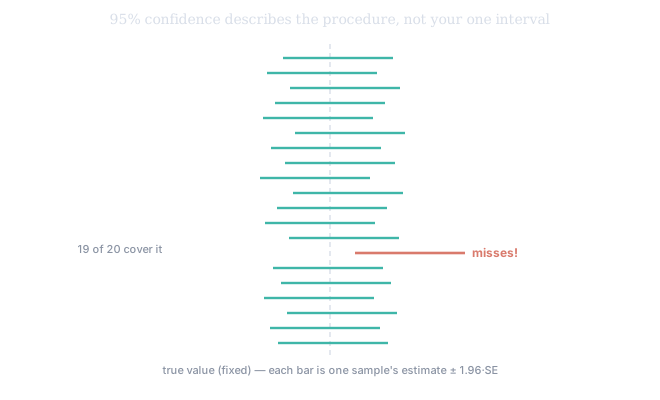
Figure 3. Twenty samples, twenty intervals, one fixed true value. About nineteen of the twenty contain it; one misses entirely. You never know which kind you drew. "95% confidence" is a property of the factory that stamps out intervals, not a probability about the single interval in your hand. A cleaner way to feel it (Wasserman's): if every day you build a 95% interval for a different, unrelated quantity, then over a long career about 95% of all those intervals will have been right.
The distinction sounds pedantic until the day you bet real money on having understood your own uncertainty, at which point it becomes the difference between humility and ruin.
The lookback tradeoff: bias vs variance, made practical
The bias–variance decomposition is not academic — it is the daily decision behind every volatility number you read, through the lookback window: how many days of history do you average over?
A short window (say 5 days) uses only the most recent, most relevant data — so it has low bias, it tracks the current regime — but it's built from few points, so it has high variance: it's jumpy and noisy. A long window (say 250 days) averages away the noise — low variance, beautifully stable — but it drags in stale history from regimes that may no longer apply, so it has high bias: it's smooth but laggy, and slow to react when the world changes. Neither extreme is right; the best window minimizes total error, MSE = bias² + variance.
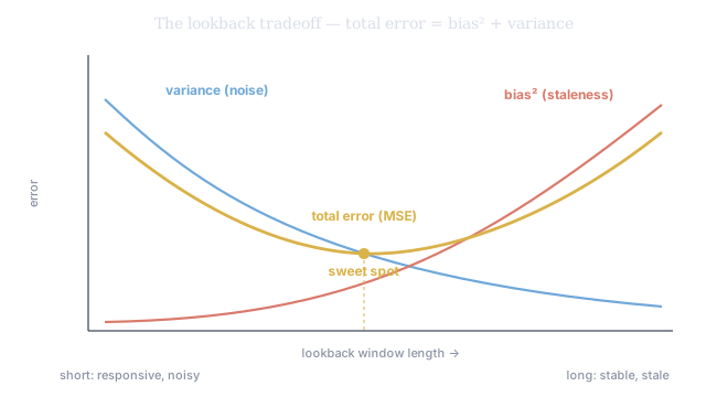
Figure 4. As the window lengthens, variance (noise) falls but bias (staleness) rises, and total error is U-shaped with a sweet spot in the middle. This is the exact tradeoff behind SV's HV(P&R) dual lookback windows: the short window for responsiveness, the long one for stability, read together so you can see both the regime and the noise around it.
When formulas fail: the bootstrap
For the sample mean, the standard-error formula is easy. For volatility, correlation, percentiles, and most things you actually care about, the formulas are hard or don't exist. Enter the bootstrap, one of the most beautiful ideas in modern statistics: instead of deriving the sampling distribution, you simulate it. Resample your own data — draw days at random, with replacement, to build a new fake sample the same size as the real one — recompute the statistic, and repeat thousands of times. The spread of those thousands of recomputed estimates is your standard error, and their middle 95% is your confidence interval — read straight off the data, no formula required. You will lean on the bootstrap throughout the institute because it works exactly where the textbook formulas give up.
One level deeper sits the general principle behind most of the estimators you'll meet later — maximum likelihood: choose the parameter value that makes the data you actually observed most probable. It's how the Student-t degrees-of-freedom from Chapter 2 get fitted, and how the GARCH and option-pricing models of the advanced tiers are calibrated. For now, just know the name and the idea: the best estimate is the one under which reality looks least surprising.
The honest close
We can now complete the definition of evidence this course has been building. Chapter 4 said a number is evidence only relative to a base rate and the noise. Add the third piece: a number is evidence only when it arrives with its uncertainty attached. A volatility of 22% give-or-take one point is a sharp claim you can act on. The same 22% give-or-take nine points is barely a claim at all. Same headline; completely different evidence. The figure on the screen is half the story — the error bar is the other half, and the screen almost never shows it to you. Your job is to always ask for it.
Any single statistic in SVQ — a volatility, a mean, a correlation — moves when computed over two different lookback windows, and that movement is the sampling distribution made visible. SV's HV(P&R) builds this in, with its short and long windows and its ±1 SE bands — the standard error drawn right on the chart, Figure 1 in the wild. Wide bands mean the estimate is uncertain and position size should reflect it; short and long windows that disagree are the bias–variance tradeoff of Figure 4 in real time. And the percentile / rank views answer not just "what is it?" but "where does this estimate sit in its own history?"