Randomness, Noise, and the Base-Rate Trap
Objectives
- Explain why a pure random walk produces convincing chart structure, and define signal vs noise.
- State and apply conditional probability and independence, and spot the gambler's fallacy.
- Distinguish P(A|B) from P(B|A) and apply Bayes' theorem to update a base rate into a posterior.
- Recognize data-snooping / multiple testing as manufactured significance, and the Law of Large Numbers as the antidote.
- Combine hit rate and payoff into expectancy, and judge a signal by how far it beats its base rate.
Here is an experiment you can run in your head. Take a coin, flip it a few hundred times, and each time it lands heads you step up one unit, tails you step down one. Plot the running total. What you get will not look like random scribble. It will look like a market. It will have trends that run for a while, levels it seems to bounce off of, breakouts and reversals — all the shapes a chart-reader lives by. And every bit of it came from a fair coin with no memory and no intention whatsoever.
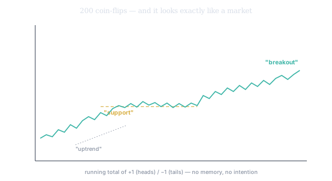
Figure 1. A cumulative path of fair coin-flips — and it has everything: an "uptrend," a "support" level it touches three times, a "breakout." None of it is real. The path is just the running sum of steps. This is the same object as the cumulative log-returns from Chapter 1: a random walk, with independent steps. Its center stays at zero, but its range drifts outward like — and that aimless wandering is what your eye insists on reading as intention.
This is the first hard lesson of inference, and it is uncomfortable: a pure random walk produces convincing structure. Our brains are pattern-finding engines that evolved to see a predator in the rustling grass, and they do not switch that machinery off when we point them at a price chart. We see support, resistance, and momentum in sequences that contain none of those things, because the absence of pattern is something the human mind is almost incapable of perceiving. The technical word for seeing patterns in noise is apophenia, and on a trading screen it is not a quirk — it is a tax you pay on every decision unless you actively defend against it.
So the central skill is separating signal from noise. Signal is the part of a movement driven by something real and, at least in principle, repeatable. Noise is the part that is just the coin-flips — the random jostling that means nothing and predicts nothing. Most of what happens on short timescales is noise. This is not cynicism; it is the starting assumption a professional brings to the screen, and the burden of proof sits on any claim that a given wiggle is more than chance. To discharge that burden you need the actual machinery of probability — so let us build it, carefully, because the rest of your statistical life rests on it.
Probability, in one paragraph of honesty
A probability is a number between 0 and 1 attached to an event — and the interpretation we will lean on is the long-run frequency one: the probability of an event is the fraction of times it would occur if you could repeat the situation forever. A fair coin has because in a long run of flips, half come up heads. Everything else — conditional probability, Bayes, the whole edifice — is built from this one idea and a couple of rules for combining events. Two events that can't both happen are disjoint, and then their probabilities add. The complement rule, , is the most useful single line in practical probability ("at least one" problems are almost always easier solved as one-minus-none).
Independence, and the gambler's fallacy
Two events are independent when knowing one tells you nothing about the other. Formally,
Coin flips are the canonical example: the coin has no memory, so each flip is independent of every flip before it. This is the death of the gambler's fallacy — the belief that after five heads in a row, tails is somehow "due." It is not. The probability of heads on the next flip is still exactly ; the coin does not know or care what just happened. The five-head streak felt meaningful, but a streak of five is precisely the kind of structure randomness manufactures all the time (look again at Figure 1). On a trading screen the same fallacy wears a suit: "it's closed up eight days running, it must pull back." Maybe it will — but not because eight up-days creates an obligation. If the moves were independent, the streak carries no information at all. (One careful note: independence has to be checked or assumed, never read off a picture — and "can't happen together" is the opposite of independent, not the same as it.)
Conditional probability: the fraction within
Most real questions are conditional — not "how likely is a crash?" but "how likely is a crash given that my signal just fired?" The conditional probability of given is
which you should read as exactly what it says: among all the times happens, what fraction also have ? You narrow the world down to the cases and ask how often shows up inside that narrowed world.
Here is the single most expensive confusion in all of applied probability, and it has its own name:
These are different questions with different answers, and people swap them constantly. The probability of spots given you have measles is essentially 1; the probability you have measles given that you have spots is nowhere near 1 (spots have many causes). In a courtroom, confusing "probability of this DNA match if innocent" with "probability of innocence given the match" has convicted innocent people — which is why this swap is called the prosecutor's fallacy. In markets it sounds like: "every major crash was preceded by this pattern!" — which is , and tells you almost nothing about what you actually need, . The pattern may also precede a hundred non-crashes.
Bayes' theorem: turning a base rate into a belief
To get from the question you can measure, , to the question you care about, , you need two more ingredients. The first is the law of total probability: to get the overall chance of , add up the ways can happen across a partition of the world,
The second is Bayes' theorem itself, which is just the conditional-probability definition applied twice:
The vocabulary matters: is the prior — what you believed before the evidence — and is the posterior — your updated belief after. And the prior, in almost every real problem, is the base rate. This is the whole chapter in one sentence: Bayes' theorem is the machine that combines the base rate with the evidence, and if you leave the base rate out, the machine gives you a confidently wrong answer.
The example that should unsettle you
A disease affects 1% of people. A test is "90% accurate": it catches 90% of sick people, and it correctly clears 90% of healthy people. You test positive. What is the chance you are sick? Almost everyone — including, in studies, most doctors — says about 90%. Let's just count, using a population of 1,000.
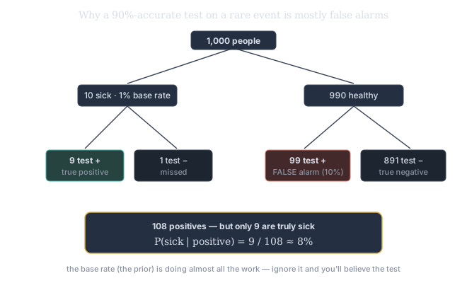
Figure 2. Count the people, don't trust the intuition. Of 1,000 people, the 1% base rate means 10 are sick and 990 are healthy. The test flags 90% of the 10 sick → 9 true positives. But it also wrongly flags 10% of the 990 healthy → 99 false positives. So 108 people test positive, and only 9 of them are actually sick: .
Eight percent. The test is genuinely 90% accurate, and a positive result still leaves you more than 90% likely to be fine — because the disease is rare, and 10% of a big healthy population is a flood of false alarms that drowns the handful of true ones. The base rate did almost all the work. Remove it from your thinking and you are off by more than a factor of ten.
The same trap, wearing a ticker
Now translate it. A "crash signal" fires before turbulent weeks. Suppose big weekly drops are rare — a 10% base rate — and the signal is even better than the medical test: it fires on 80% of real crash-weeks and false-fires on only 20% of calm weeks. Your signal lights up. How worried should you be? Count 1,000 weeks: 100 are crash-weeks → the signal catches 80; 900 are calm → it false-fires on 180. The signal fired 260 times, but only 80 were real:
An "80% accurate" crash signal is wrong more than two times out of three when it fires, because crashes are rare to begin with. There is a quick way to see this without the full table — Bayes in odds form: posterior odds prior odds likelihood ratio. Here the prior odds are , the likelihood ratio is , so the posterior odds are — that is . Same answer, ten seconds of arithmetic. This is what we meant in the abstract earlier when we said a signal is only worth the amount by which it beats its base rate. Bayes is the tool that measures the beating exactly.
Manufactured patterns: noise bands and data-snooping
Two more ways randomness fools you, because both run rampant in trading research.
First, a measured relationship is never exactly zero on noise. If you compute the correlation between a pattern and tomorrow's return on finite data, pure chance gives you a number that wobbles around zero with a standard error of roughly . So any apparent signal smaller than about is indistinguishable from noise — that band is the white-noise envelope, and a "discovery" inside it is nothing. With 100 observations that band is a wide ; a lot of celebrated "edges" live entirely inside it.
Second, and more insidious: data-snooping, the multiple-testing trap. If you test one rule at the 5% significance level, there's a 5% chance it looks good by luck. But test twenty unrelated rules and the expected number that look "significant" by pure chance is . So finding one winner among twenty you tried is exactly what noise predicts — it is evidence of nothing.
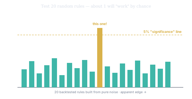
Figure 3. Twenty trading rules built from pure noise, backtested. Nineteen show the small random "edges" you'd expect; one happens to clear the significance line. If you only report that one — "look, this rule works!" — you have manufactured a discovery out of randomness. This is why a dazzling backtest, on its own, is not evidence. The honest question is always: how many things did you try before you found this one?
The Law of Large Numbers: the antidote
If randomness is so good at faking signal, how does the truth ever surface? Through the Law of Large Numbers (LLN), one of the deepest results in probability. It says that as you collect more independent observations, the sample average converges to the true mean:
The fraction of heads in a long run of flips piles up tightly around ; the average outcome of a strategy with a real edge piles up around its true expectation. This is the casino's entire business model — each spin is nearly a coin-flip, but over millions of spins the house's tiny edge becomes a mathematical certainty.
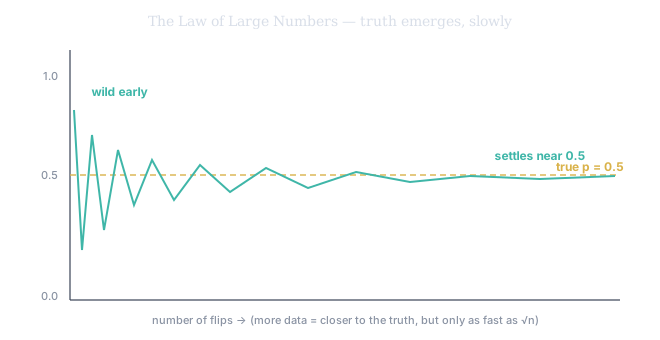
Figure 4. The running proportion of heads. Early on it swings wildly — a few flips prove nothing, and a 70%-heads start is common. As the flips accumulate, it settles toward the truth. But notice how slowly: the noise around the truth shrinks only as — the same you met as the standard error in Chapter 3. To halve your uncertainty you need four times the data.
That slowness is the catch, and it is the bridge to everything ahead. The LLN guarantees the truth emerges eventually, but "eventually" can mean hundreds or thousands of independent trades. A handful of winning trades is not evidence of an edge — it is a 70%-heads opening streak. This is why a real verdict on "did this beat chance?" requires a formal hypothesis test, the first thing you build in Tier 200. For now, hold the discipline: trust convergence, distrust streaks.
Hit rate is not edge: expectancy
One final synthesis, because base-rate thinking has a profitable twin. Even a signal that genuinely beats its base rate can lose money, and a signal that's wrong most of the time can mint it — because what you actually bank is expectancy, the probability-weighted average outcome you met as expectation in Chapter 3:
A system that wins only 40% of the time but makes on a win and loses on a loss has expectancy per trade — strongly positive. A system that wins a comforting 90% of the time but occasionally gives back to pocket has expectancy — a slow bleed dressed up as a winning record. The high-hit-rate system is exactly the negatively-skewed, fat-left-tail profile from Chapter 2: calm, calm, calm, ruin. Hit rate is the part of the story your base-rate-blind intuition fixates on; payoff is the part that pays. You need both, multiplied.
The honest summary
A number on the screen is evidence only relative to three things: the base rate of the event it claims to predict (the prior Bayes multiplies in), the noise band it has to rise above, and the number of alternatives that were tried before it was found. A reading that doesn't clear all three is not a signal — it's a coin-flip wearing a decimal point and a confident name. The defenses are concrete: count the people (Bayes), distrust streaks (LLN), ask how many rules were tested (data-snooping), and judge a system by expectancy, not hit rate. This is the statistical conscience the rest of the program will sharpen into formal tools.
Every indicator Saqrid surfaces carries the same Bayesian question before any action: what's the base rate of the move it predicts, and what's its hit rate when it fires? With those two numbers in hand, the odds-form update — prior odds × likelihood ratio — works exactly as in Figure 2's crash-signal box. If the posterior isn't well above the base rate, the signal is noise. The research behind it faces the same scrutiny: was this rule found alone, or cherry-picked from twenty? And every claimed edge reads against SV's HV(P&R) standard-error bands — inside the band is inside the noise.