Center and Spread: Mean, Variance, Volatility
Objectives
- Compute and interpret the mean (as an expectation), median, variance, and standard deviation of a return series.
- Use robust measures — median, MAD, IQR — and explain why fat tails make the ordinary mean and standard deviation unstable.
- Define volatility as the standard deviation of returns and annualize it correctly with the √time rule, knowing the assumption it smuggles in.
- Read covariance and correlation as the first cross-moment, and write the variance of a two-asset portfolio.
Every distribution you will ever look at can be squeezed, imperfectly, into two questions. Where does it sit? And how widely does it spread? In the last chapter you learned to see the whole shape of a return distribution. Now you learn to summarize it in a few numbers — and, just as importantly, to know exactly what those numbers quietly throw away. This is the chapter where the word volatility finally gets a precise definition, because volatility is nothing more exotic than the spread of returns, measured carefully.
The center: the mean, and the expectation behind it
The most common measure of center is the mean, the simple average: add up every return and divide by how many there are. The mean is the balance point of the histogram — the spot where the picture would sit level on a fingertip.
It is worth naming what the mean really is, because the idea generalizes. The mean is an expected value, written — the probability-weighted average of all the values the variable can take. For a sample it is just the arithmetic average; for a distribution it is each outcome weighted by how likely it is. The reason this matters is one beautiful property called linearity of expectation:
The expected value of a sum is the sum of the expected values — always, whether or not the pieces are related to each other. This is the quiet workhorse behind all of portfolio math: the expected return of a portfolio is just the weighted average of its holdings' expected returns, no matter how tangled their relationships. Hold that thought; it breaks in an instructive way when we get to risk.
But the mean has a weakness you already half-know from the last chapter. It is exquisitely sensitive to the tails. One enormous crash, one violent rally, drags the mean toward itself far more than its single day of existence should warrant. On a fat-tailed, skewed series — that is, on almost every real asset — the mean is not the return you experience on a normal day. The everyday return, the one in the thick middle of the histogram, is better captured by the median: the value that splits the data in half, with as many days above as below. When the mean and the median pull apart, that gap is itself information — it is the fingerprint of skew. A mean well below the median says the left tail is doing the dragging. Never quote a mean for financial returns without glancing at the median beside it.
When the tails lie: robust center and spread
The mean's fragility is not a quirk; it is a direct consequence of the fat tails you measured in Chapter 2. And it infects the spread too. So practitioners keep a second toolkit of robust estimators — measures built to ignore the outliers rather than be hijacked by them.
For the center, that is the median. For the spread, the two standard robust tools are the interquartile range (IQR — the distance between the 25% and 75% quantiles, the width of the "middle half" of the data) and the median absolute deviation (MAD — the median of how far each point sits from the median, scaled so that on clean normal data it matches the standard deviation).
Here is why this is not academic. On daily S&P 500 log-returns, the ordinary sample standard deviation is about 0.011, while the MAD-based estimate is 0.0079 — markedly smaller. Same data, two answers. The standard deviation is inflated by a handful of crash days; the MAD looks past them at the typical day. Neither is "wrong," but they answer different questions, and the gap between them is itself a thermometer for fat tails: when your robust and non-robust spread estimates disagree this much, the data is telling you it is not normal. The need for robust estimators is itself a sign of nonnormality.
The spread: variance and standard deviation
Now the spread proper. The center tells you nothing about risk; risk lives in the scatter. We measure it by asking, on average, how far each return falls from the mean. But there is a subtlety: deviations above and below the mean cancel if we just average them — by construction they sum to zero. So we square each deviation first. Squaring does two useful things at once: it kills the sign, so nothing cancels, and it punishes large misses far more than small ones — exactly what we want when the large misses are the ones that hurt. The average of those squared deviations is the variance:
Variance has one inconvenience: because we squared, it lives in squared units — squared returns — which no human can intuit. So we take the square root and return to the original scale. That square root is the standard deviation .
Two properties of variance will repay you for the rest of the course. First, the scaling law: for constants ,
Adding a constant (a guaranteed return) changes risk not at all; scaling by changes variance by and therefore standard deviation by . Double your position size and you double your volatility but quadruple your variance — the asymmetry that makes leverage so treacherous. Second, for independent pieces, variances simply add:
Remember that linearity of expectation worked for any sum? Variance does not — it only adds cleanly when the pieces are independent. That single asterisk is where all of risk management lives, and we return to it at the end of the chapter.
One technical note you will see in every formula: when you estimate variance from a sample you divide by , not . The sample mean is itself fitted from the data, using up one "degree of freedom," and dividing by corrects for it so that, on average, the estimate hits the true variance: . It is a small honesty adjustment, but it is why your spreadsheet's STDEV and STDEV.P give slightly different answers.
Volatility = the standard deviation of returns
In finance the standard deviation of returns has a name you already know: volatility. When someone says an asset "has a volatility of twenty percent," they mean the standard deviation of its returns, expressed on an annual basis, is twenty percent. Volatility is the single most important number in this course, because nearly everything downstream — option prices, risk limits, position sizing — is built on it.
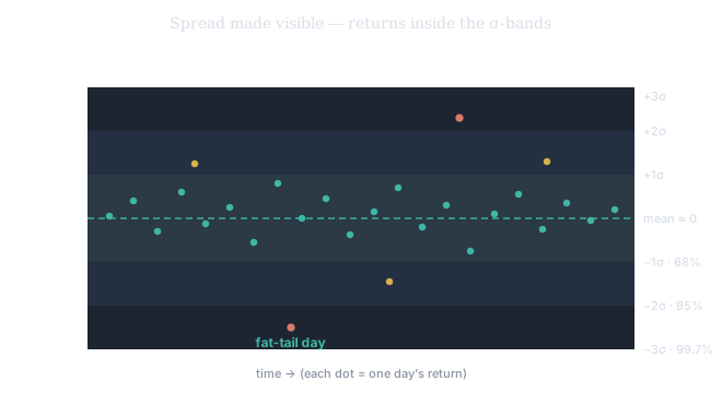
Figure 1. Volatility, drawn. Each dot is a day's return scattered around a near-zero mean; the shaded rings are ±1σ, ±2σ, ±3σ. On a well-behaved series most days land inside ±1σ (about 68%), almost all inside ±2σ (about 95%). The fat-tail days that punch beyond ±2σ (red) are exactly the ones Chapter 2 warned you arrive more often than the bell curve allows. These bands are the skeleton of SV's Normal Expected Move — the σ-ladder a trader reads off a chart.
Annualizing: the square-root-of-time rule
That phrase "on an annual basis" hides one last operation you must get right. Volatility is usually computed from daily returns but quoted annually. To convert, use the square-root-of-time rule: multiply the daily volatility by the square root of the number of trading days in a year — about . A daily volatility of 1% becomes an annual volatility of roughly 16%.
Why the square root, and not the number itself? Because of the variance-additivity law above. If daily returns are independent draws from the same distribution, the variance over days is times the daily variance, so the standard deviation — being the square root — grows like :
Risk grows with the square root of time, not linearly. The naive instinct — "ten days is ten times as risky" — overstates it badly.
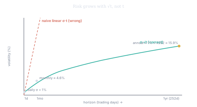
Figure 2. The correct √t curve (teal) rises steeply at first and then flattens; naive linear scaling (red) shoots off the chart. Daily 1% → monthly ≈ 4.6% → annual ≈ 15.9%. The whole annualization convention is this one curve.
The same shows up in a place that explains an earlier puzzle. How well do you know the mean? The standard error of the sample mean is
which shrinks only as fast as . Because daily volatility utterly dwarfs the daily mean return, you would need an absurd number of observations to pin the mean down — which is the deep reason we said the mean is a poor, noisy summary while volatility is estimable and trustworthy. Spread you can measure; center you can barely see.
And here is the honest caveat that ties this chapter back to the last. The √time rule assumes returns are independent and identically distributed — each day a fresh, unrelated draw from the same distribution. You already know that is false: volatility clusters; turbulent days arrive in groups. So annualized volatility is a useful convention, not a law of nature, and it understates risk precisely during the storms when clustering is strongest. Quote it, use it, but never forget the assumption you smuggled in to get it.
The first cross-moment: covariance and correlation
So far, one asset at a time. But the deepest idea in portfolio risk is about pairs — how two assets move together. The measure is the covariance:
When the two tend to be above their means on the same days (and below on the same days), the product is positive on average and the covariance is positive — they move together. When one is up while the other is down, the covariance is negative. Covariance is the first cross-moment: the second moment () measured across two variables instead of one.
Covariance has the same units problem as variance, and worse — it scales with both assets. So we standardize it into the correlation:
Correlation is unitless and bounded: is perfect lockstep, is perfect opposition, is no linear relationship. One crucial caution: independence implies zero correlation, but zero correlation does not imply independence — two variables can be tightly, nonlinearly related and still show . (That gap is exactly why Tier 400 reaches past correlation to copulas, which capture how assets crash together even when ordinary correlation looks calm.)
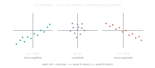
Figure 3. Correlation is a shape. Plot two assets' daily returns against each other: a tight up-sloping cloud is high positive ρ, a round blob is ρ ≈ 0, a down-sloping cloud is negative ρ. This is the picture behind every diversification and hedging decision.
Now we collect the reward. The variance of a two-asset portfolio is not just the sum of the two variances — the cross term appears:
This single line is the seed of diversification. When , the covariance term is smaller than it would be in lockstep, so the combined risk is less than the sum of the parts — you got risk reduction for free by holding things that don't move identically. And it warns you of the trap: in a crisis correlations rush toward , the cross term swells, and the diversification you were counting on evaporates exactly when you need it. That failure mode — correlations going to one in the tail — is the through-line into the contagion and regime tools of the advanced tiers.
The honest summary
A distribution becomes a handful of numbers: a center (mean — or, when the tails lie, the median), a spread (variance and its square root, volatility — or the robust MAD), and, for pairs, a co-movement (covariance and correlation). Volatility is the standard deviation of returns; it annualizes by under an i.i.d. assumption you know to be optimistic; and the moment you hold more than one asset, the correlation between them governs your real risk more than either volatility alone. Every number here has a place it lies — and knowing where is the whole skill.
SVQ's realized/annualized volatility readout is this chapter's arithmetic: the standard deviation of an asset's daily log-returns, multiplied by √252, lands within rounding distance of it — a number once taken on trust becomes one that can be derived. SV's Normal Expected Move overlay is Figure 1 come alive: the ±1σ/±2σ bands drawn straight on the chart. And SVQ's correlation between two assets raises the question that matters most — what happens to that number on the worst days. The answer is the difference between a portfolio that diversifies and one that only looked diversified.