Non-Parametric Tests & Percentiles (HVP / HVR)

Everything you have done so far in this course leaned, somewhere, on a number's magnitude — how far a mean sat from zero, how many standard deviations a value was out in the tail. That works beautifully when the data behaves. The trouble is that financial data so often does not: volatility clusters, returns have fat tails, and a single crisis day can drag a mean and inflate a variance until your tidy parametric test is quietly lying. So this final chapter of the inference tier asks a different question — what if you threw away the magnitudes entirely and kept only the order?

The rank

That is the whole idea behind rank-based, or non-parametric, methods. Sort your numbers and replace each value with its position in the sorted list: smallest is rank 1, next is rank 2, up to the largest at rank $N$ . A wild outlier of +50, which would have detonated an average, becomes merely "the biggest one" — rank $N$ , no more influential than if it had been +5. You trade the exact distances between values for something robust and distribution-free: ranks do not care what shape the data came from.

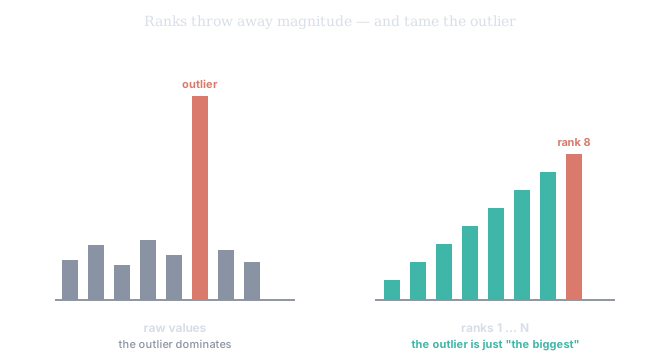
*Figure 1.* The same data twice. As **raw values** (left) one outlier towers over everything and would dominate any mean or variance. As **ranks** (right) that outlier is just rank $N$, one step above its neighbor. Ranking is a deliberate act of throwing away magnitude to buy immunity from outliers — exactly the immunity fat-tailed markets demand. — *Figure 1.* The same data twice. As **raw values** (left) one outlier towers over everything and would dominate any mean or variance. As **ranks** (right) that outlier is just rank $N$ , one step above its neighbor. Ranking is a deliberate act of throwing away magnitude to buy immunity from outliers — exactly the immunity fat-tailed markets demand.

The percentile and the quantile

The most useful thing you build from ranks is a percentile — today's value located inside its own history. Its percentile is the fraction of past observations at or below it:

$\text{percentile}(x) = \frac{k}{N}\times 100, \qquad k = \#\{\text{observations below } x\}.$

If today beats 900 of the last 1,000 days, it sits at the 90th percentile. Read that twice: the 90th percentile does not mean the value is large in any absolute sense — it means large relative to its own past, unusual for this asset by this asset's own standards.

One careful note, because the sloppy version causes off-by-one errors. Counting " $\le x$ divided by $N$ " for a value inside its own sample can never be zero (every value is $\le$ itself) and maps the single largest observation to 100% — the maximum reported as beating itself. So state a convention: the strict-below count matches the intuition above; the common library default is the mid-distribution (Hazen) estimator, which counts those below and adds half of any ties. Either is fine; silently mixing them is what bites. Going the other way — from a percentile back to a value — gives a quantile: the 50th percentile is the median, the most robust center you own, completely indifferent to tail fatness.

HVP and HVR

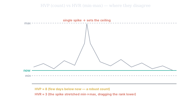
*Figure 2.* A year of historical volatility with one big spike, and current vol sitting low. **HVP** (percentile) counts the fraction of days below now — a robust ~8. **HVR** (min-max rank) places now on the floor-to-ceiling scale — but the lone spike stretched the ceiling, so HVR reads even lower, ~3. Same state, two honest answers to two different questions.

In Saqrid

This is exactly what SVQ's HVP and HVR give you. HVP, the historical-vol percentile, reports where current realized vol falls in its trailing window — the $k/N$ count you just learned; an HVP of 5 means vol is lower than 95% of the lookback, crushed. HVR, the historical-vol rank, is the min-max version: it places current vol on a 0–100 scale stretched between the window's lowest and highest readings. The distinction matters: HVP only counts, so it is robust; HVR measures position between floor and ceiling, so it is sensitive to a single extreme day that sets the ceiling. When both read low together, rank-based and range-based methods agree this asset is unusually quiet — and quiet, for a trader hunting expansion, is a setup worth respecting. Both are non-parametric, which is why they're more honest than a sigma-based z-score on fat-tailed vol.

Testing with ranks: Wilcoxon

Ranks let you test, not just describe. To ask whether volatility this month genuinely differs from last month — without a normality assumption fat-tailed vol will violate — use the Wilcoxon rank-sum test (a.k.a. Mann-Whitney U). Pool both samples, rank every observation together as one list, and sum the ranks belonging to the first group:

$W = \sum_{i \in \text{group 1}} \text{rank}(x_i).$

If the two groups came from the same distribution, $W$ lands near its chance expectation; if group one systematically out-ranks group two, $W$ drifts far out and yields a p-value the usual way. The paired cousin, the Wilcoxon signed-rank test, ranks the absolute differences and re-attaches their signs — a robust replacement for the paired t-test. The move is the one you've now seen repeatedly: convert magnitudes to ranks, and let the ordering carry the evidence.

The permutation test: let the labels build the null

There is a deeper, almost magical, distribution-free test — and it is the perfect capstone for this tier. Suppose you have two groups and a statistic measuring their difference (say, the gap in medians), $T_{\text{obs}}$ . Here is the key idea: if the null is true — the two groups come from the same distribution — then the group labels are arbitrary. Which observation got called "A" and which "B" was a coin flip that carries no information. This property is called exchangeability, and it hands you the null distribution for free.

So you manufacture it. Pool all the observations, randomly reshuffle the A/B labels, recompute the statistic $T^*$ on the relabeled groups, and repeat thousands of times. The spread of those $T^*$ values is exactly what the difference would look like if the labels truly meant nothing — the permutation null distribution. Your p-value is just how often a shuffle is as extreme as what you actually saw:

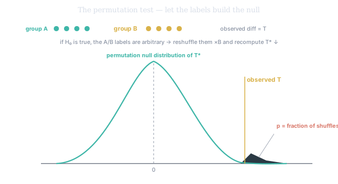
$p = \frac{1}{B}\sum_{b=1}^{B}\mathbf{1}\big\{\,|T^*_b| \ge |T_{\text{obs}}|\,\big\}.$

*Figure 3.* Reshuffle the labels many times, recompute the difference each time, and you get the null distribution centered at zero. The observed difference sits far in its tail, so few shuffles match it — a small p-value, with **no formula and no distributional assumption anywhere.** The data built its own reference distribution.

Robustness vs power — and the two pillars

The honest caveat, so you're not over-sold: throwing away magnitudes throws away information. When the data genuinely is well-behaved and normal, a parametric test is more powerful — it will catch a true effect a rank test might miss. Non-parametric methods are what you reach for when you don't trust the distribution, which in markets is most of the time. You buy robustness and pay with a little power, and knowing you're making that trade is the mark of someone who reads a percentile as evidence, not decoration.

Step back and notice what closes this tier. Two computational ideas have done the heavy lifting wherever formulas failed: the bootstrap of ch2 and the permutation test here. They are siblings — both abandon assumption-laden formulas and let the data generate its own reference distribution — distinguished by purpose. The bootstrap resamples with replacement to estimate a sampling distribution (a standard error, a confidence interval). The permutation test reshuffles labels without replacement to build a null distribution (a test, a p-value). Together with maximum likelihood (ch1), confidence intervals (ch2), and hypothesis tests (ch3), you now hold the full engine of statistical inference. Tier 200's next course, SVI 202, points it at relationships — regression and time series, and the GARCH volatility models the EWMA only previewed.