Prices, Returns, and Why We Use Log-Returns
Objectives
- Compute simple (arithmetic), gross, and multiperiod returns from a price series, and annualize them.
- Explain why arithmetic returns are asymmetric and do not add cleanly over time.
- Derive the log-return from continuous compounding and state its two key properties: time-additivity and symmetry.
- State the one place log-returns fail — aggregation across a portfolio — and know which scale to use when.
- Recognize when the platform is working in log space and why every statistic downstream depends on it.
A price, by itself, tells you almost nothing.
If I tell you an asset is trading at four hundred and twelve, you cannot do anything with that. Is that expensive? Cheap? Up or down? A price is a label, not a measurement.
The information — the thing you can reason about, compare across assets, and feed into a model — is the change. Finance is not built on prices. It is built on returns. The textbook reason, due to Campbell, Lo, and MacKinlay, is twofold: a return is a complete, scale-free summary of an investment (a 2% gain means the same thing on a five-dollar stock and a five-thousand-dollar one), and return series have far better statistical properties than prices — they sit still long enough to be modeled, in a sense we will make precise over the next few chapters.
So let us define a return carefully, because the careless version costs real money.
The simple return and the gross return
The simple return, sometimes called the arithmetic return, is the change in price over a period divided by where you started. If the price was one hundred yesterday and is one hundred and ten today, the return is ten divided by one hundred, or ten percent.
Written out, the simple return from one period to the next is the new price minus the old price, all over the old price — equivalently, the new price divided by the old, minus one:
That ratio of new to old — one-point-one, in our example — is called the gross return:
The gross return is what you multiply your money by; the simple return is the gross return with the one stripped off, so it reads as a percentage gain or loss. Keep both in mind — the gross return is the natural object when you compound, the net return when you report.
All of this is intuitive, and for a single period it is exactly right. The trouble begins the moment a second period arrives, because simple returns conceal two traps.
Trap one: asymmetry
The first trap is asymmetry. Suppose you lose fifty percent. How much do you need to gain to get back to even?
Most people's gut says fifty percent. The real answer is one hundred. Start at one hundred and lose half, and you stand at fifty; a fifty percent gain from there lifts you only to seventy-five. To climb all the way home, the fifty has to double.
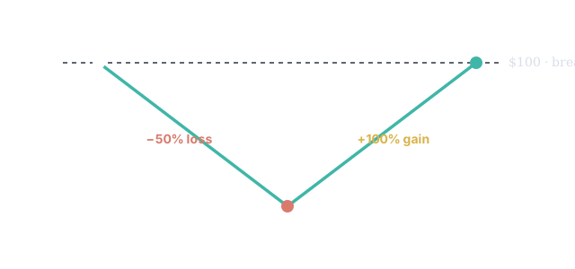
Figure 1. Losses and gains of the same percentage are not mirror images: a 50% loss must be undone by a 100% gain.
Losses and gains of the same percentage are not mirror images. A minus-ten and a plus-ten do not cancel — start at 100, drop 10% to 90, rise 10% to 99; you have lost a dollar by going nowhere. This asymmetry quietly corrupts any analysis that treats returns as if they live on a symmetric scale — averaging them, laying them on a normal distribution, computing a standard deviation — and a great deal of analysis does precisely that.
Trap two: simple returns do not add across time
The second trap is that simple returns do not add across time. If you earn ten percent one day and ten percent the next, your two-day return is not twenty percent. It is one-point-one times one-point-one, which is one-point-twenty-one — a twenty-one percent gain:
Returns compound: they multiply, they do not sum. The general rule for a -period gross return is the product of the one-period gross returns,
which is exactly why a "+10% then −10%" round trip loses money: , not . Any time you want to aggregate returns over time you are stuck multiplying gross returns — awkward on the arithmetic side and, as you will see, a swamp on the statistical one.
Annualizing: comparing returns on a common clock
Because the time interval matters, returns are usually quoted on a common annual clock. If you held an asset for years, the annualized (average) return is the geometric mean of the one-period gross returns:
A geometric mean, not an arithmetic one — because returns multiply. (For the small daily returns that dominate most series, a first-order Taylor expansion lets you approximate this by the ordinary average, , but that shortcut quietly degrades when returns get large — which is precisely when you care most.) The lesson of both traps is the same: the arithmetic scale fights you the moment time or size grows. What we need is a scale on which returns add, and on which up and down are honest mirror images.
The fix: log-returns
There is an elegant fix, and it is the reason nearly every quantitative system — Saqrid included — does its internal work not in simple returns but in log-returns.
The log-return is simply the natural logarithm of the gross return. And because logarithms turn products into sums, that is also the log of the new price minus the log of the old:
One small definition, two properties — and both traps dissolve.
Property one: log-returns add across time
The log-return over two days is exactly the first day's log-return plus the second day's. No multiplying, no compounding gymnastics — you just sum them. Over a whole window of days,
This falls straight out of the product rule: take the log of the -period compound return above, and the chain of multiplied gross returns collapses into a sum of log-returns. Want a monthly return from daily ones? Add the dailies. Want to scale a daily figure to annual? Multiply by the number of periods. This single property — that a quantity which used to multiply now adds — is why almost all time-series statistics live in log space. Sums are the native tongue of probability; means, variances, and the central limit theorem all speak it fluently, and products do not.
Property two: log-returns are symmetric
A move down and the equal-and-opposite move back up are now true negatives of each other. From 100 down to 50 is ; from 50 back to 100 is . Exact negatives, summing to zero — the scale correctly reports that you ended where you began. It no longer punishes losses on a secret, steeper schedule than it rewards gains, which means the tools you will meet later — means, variances, the normal distribution — behave themselves instead of inheriting a hidden bias.
Where the log actually comes from: continuous compounding
It is worth seeing why the logarithm shows up, because it is not a trick pulled from a hat — it is what compounding becomes when you push it to the limit.
Put one dollar in a bank at 10% per year. Paid once a year, you finish with 1.10. Paid twice a year, each half-period earns 5%, so you finish with — slightly more, because the interest itself earns interest. Paid times a year, you have . Push to infinity — interest credited continuously, drip by infinitesimal drip — and this converges to a clean limit:
So if a price grows from to under continuous compounding at rate , then , and inverting gives — the log-return. That is the whole story: the log-return is the continuously-compounded rate of return, and continuous compounding is the only compounding convention under which rates add over time instead of multiplying. The mathematics was forced; we just chose the convention that makes the algebra honest.
A bonus: they agree with simple returns for small moves
There is one more gift. For small returns the log-return and the simple return are almost indistinguishable, because when is small. The two definitions only pull apart for large moves — and when they do, they pull apart in a specific direction:
| Simple return | Log-return | Gap |
|---|---|---|
| +1% | +0.995% | negligible |
| +5% | +4.88% | small |
| +10% | +9.53% | noticeable |
| +20% | +18.2% | real |
| +50% | +40.5% | large |
| −50% | −69.3% | large |
| +100% | +69.3% | large |
For the small daily moves that dominate most series, you can read a log-return as a percentage and barely be wrong. The gap only widens for big moves — which, not coincidentally, are precisely the moves where the asymmetry trap would otherwise have bitten you. Notice the bottom rows: a +100% and a −50% have log-returns of exactly and — the symmetric pair from before, back to take a bow.
A five-day price series: 100, 102, 99, 103, 101, 104. The daily log-returns are . The five-day log-return is their sum: . Check it directly: . They match — that is time-additivity at work. (The simple returns, by contrast, would have to be multiplied as gross returns to get .)
The one caveat: log-returns do not add across a portfolio
Log-returns are immaculate across time, but you must know their one limitation, because it trips people constantly: log-returns do not add across assets. The log-return of a portfolio is not the weighted sum of its holdings' log-returns.
Here is why, concretely. Hold half your money in asset A and half in B. The portfolio's simple return is the weighted average of the simple returns:
That tidy weighting is a property of the arithmetic scale. But the logarithm of a weighted average is not the weighted average of the logarithms, so . Suppose A returns +10% and B returns −10% over the same period, equally weighted. The portfolio's simple return is exactly . But the average of the log-returns is , or about −0.5% — a different, wrong answer for the portfolio.
So there is a real trade-off, and the rule is simple to state. Across time, use log-returns: they add, and the statistics behave. Across a portfolio at a single instant, use simple returns: they weight cleanly. Each scale owns its own direction — time belongs to the logarithm, the cross-section to arithmetic — and knowing which space you are standing in is half of not making an error.
Why this matters for everything ahead
This is not a notational nicety you can forget after the quiz. Every statistic you will meet for the rest of this institute — the mean and standard deviation of the next chapter, the volatility estimators, the normal-distribution machinery, the GARCH models, the option-pricing formulas — stands on the additive, symmetric scale you just learned. Volatility is the standard deviation of log-returns. The lognormal price model that underlies Black–Scholes is precisely the statement that log-returns are normal. The probability cones Saqrid draws are log-normal projections. Get this scale right and the rest of the curriculum clicks into place; get it wrong and every downstream number inherits a quiet bias that compounds with everything built on top of it.
Every return series in SV and SVQ follows this rule. The values plotted there as "returns" are, in almost every case, log-returns — that is why a long downtrend and the rally that retraces it look proportionate on the chart rather than the rally looking deceptively larger. When the platform computes volatility, correlation, GARCH, or anything downstream, it is summing and averaging in this log space. The forward probability cone, covered later, is a log-normal projection that assumes exactly this base. That is why it was built that way: every statistic in the platform rests on the additive, symmetric scale from this chapter.